Session 4: Maps
Maps
- Useful to visualize spatial data
- Again, think of comparisons, but in space!
- Goal of this session:
- Find maps online
- Combine spatial data with other information (GDP etc.)
- Plot maps with ggplot2
Note: Complex topic, very brief overview only, if you would like to know more, let me know and we organize a separate course!
Example
Where to get maps and spatial data?
- Each map comes in a specific spatial format, the so-called “shapefile”
- Country shapefiles and subnational data can be obtained at http://gadm.org
- Useful for single country shapes
- Lower-level administrative units
- Read the downloaded file with
country_map <- readRDS("path_to_file")
Many other sources of spatial data
- Conflict data
- Uppsala Conflict Data Program GED http://ucdp.uu.se/downloads/
Generate your own!
- Measure location of interviews with a GPS device
Read spatial data in R
Note: you can find the world shapefile on the course website!
library(maptools)

world <- readShapeSpatial("./data/shapefiles/TM_WORLD_BORDERS_SIMPL-0.3.shp")

plot(world)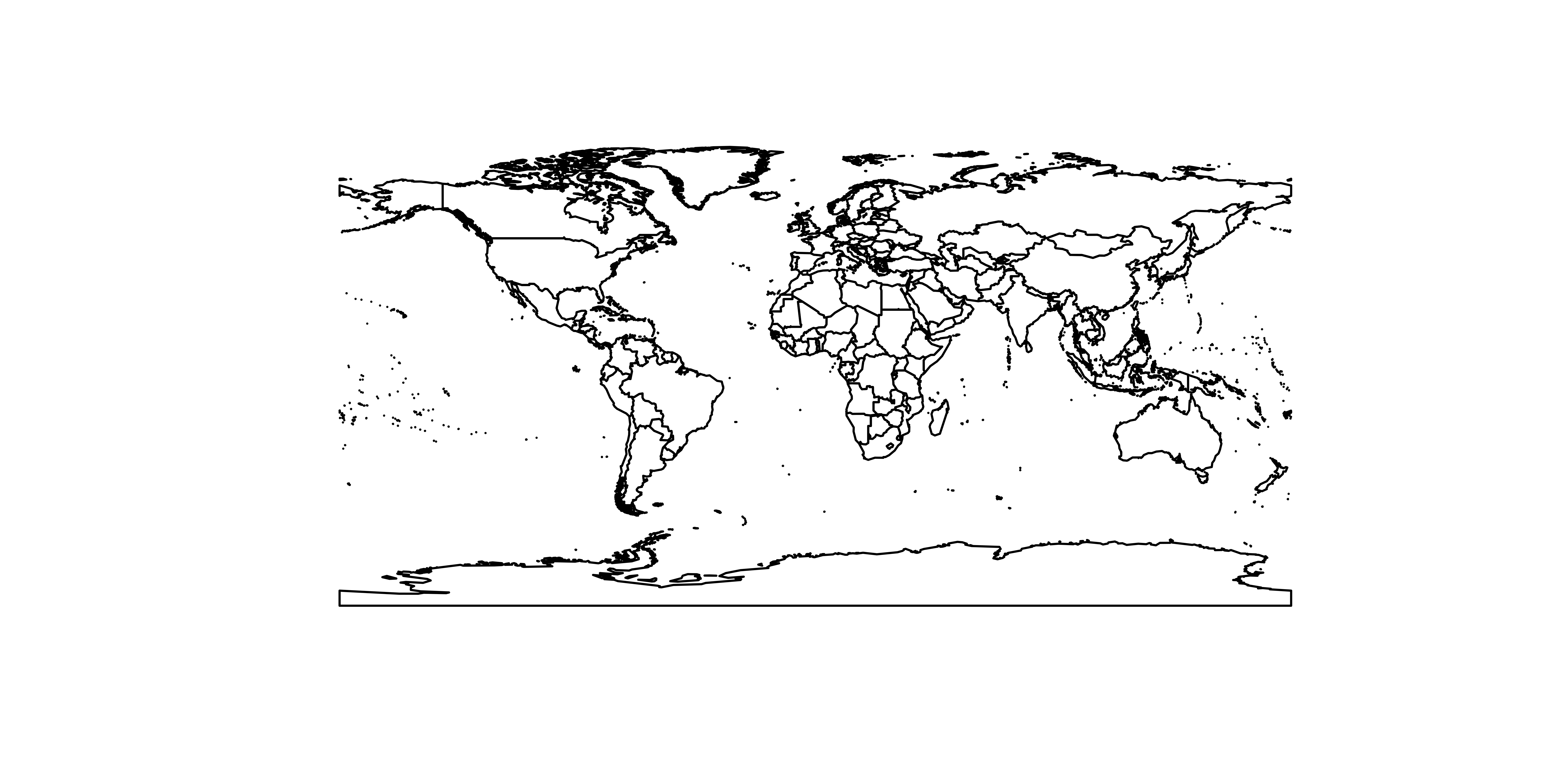
Manipulate and view spatial data
The world object from the previous slide is a special kind of data frame, a SpatialDataFrame. It works like most other data frames, but has a few quirks.
Manipulating SpatialDataFrames: countrycode()
library(countrycode)
library(maptools)

world <- readShapeSpatial("./data/shapefiles//TM_WORLD_BORDERS_SIMPL-0.3.shp")

world$continent <- countrycode(world$ISO3,
                               "iso3c", # input format
                               "continent") # output format

table(world$continent)
##
## Africa Americas Asia Europe Oceania
## 57 53 50 51 25Manipulate and view spatial data
Manipulating SpatialDataFrames: subset()
library(countrycode)
library(maptools)

world <- readShapeSpatial("./data/shapefiles//TM_WORLD_BORDERS_SIMPL-0.3.shp")

world$continent <- countrycode(world$ISO3,
                               "iso3c", # input format
                               "continent") # output format

africa <- subset(world, continent == "Africa")

par(mar=c(0.1, 0.1, 0.1, 0.1))
plot(africa)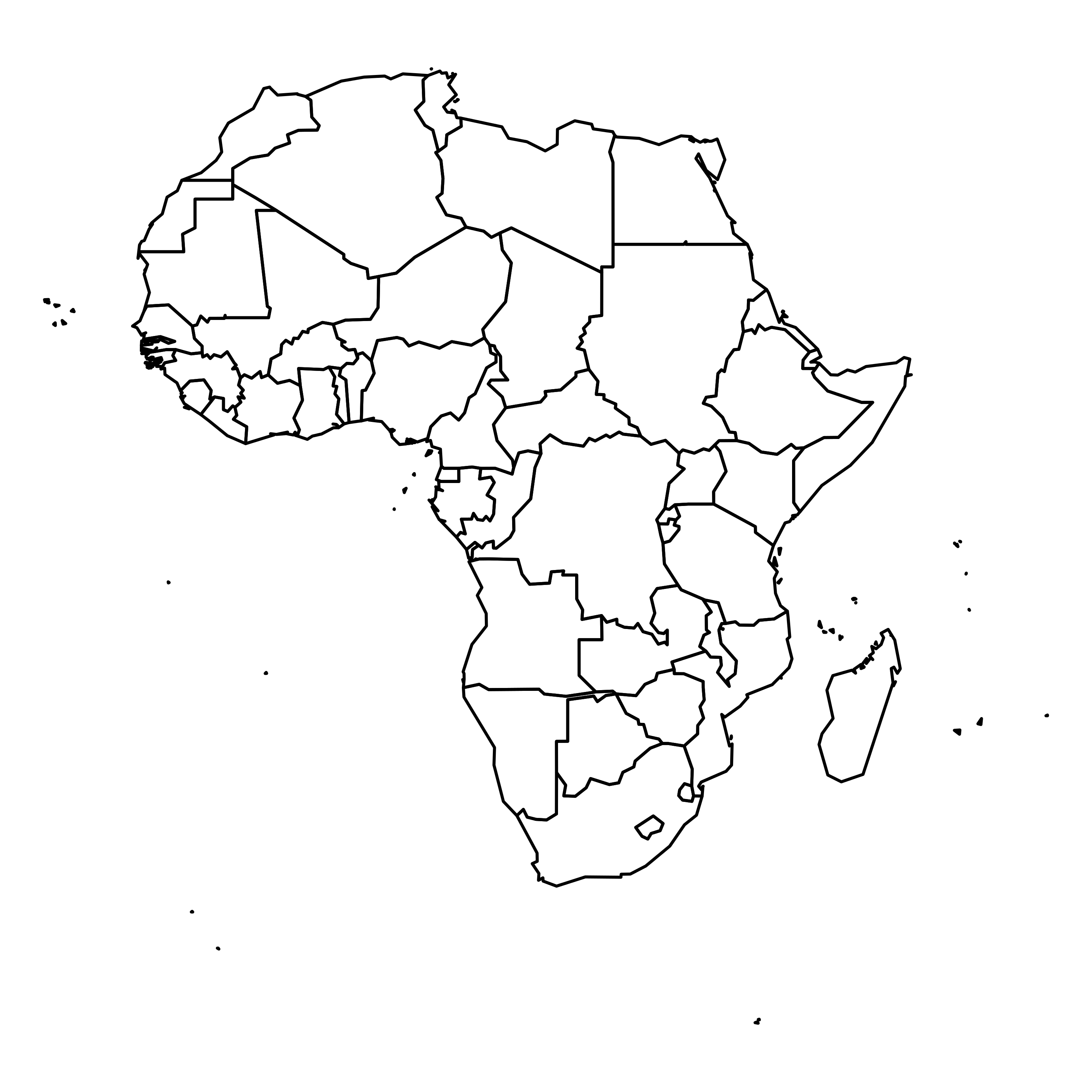
Manipulate and view spatial data
Manipulating SpatialDataFrames: View()
library(countrycode)
library(maptools)

world <- readShapeSpatial("./data/shapefiles//TM_WORLD_BORDERS_SIMPL-0.3.shp")

world$continent <- countrycode(world$ISO3,
                               "iso3c", # input format
                               "continent") # output format


View(world@data) # note the '@' as compared to other data frames
Merge in other data I
library(countrycode)
library(maptools)
library(ggplot2)
library(tidyverse)
library(gapminder)
library(broom)

world <- readShapeSpatial("./data/shapefiles//TM_WORLD_BORDERS_SIMPL-0.3.shp")

# create continent identifier
world$continent <- countrycode(world$ISO3,
                               "iso3c", # input format
                               "continent") # output format

# subset Africa shape file
africa <- subset(world, continent == "Africa")
Merge in other data II
…continued from previous slide.
# get gapminder data
data("gapminder")

# create country identifier for merging
gapminder$ISO3 <- countrycode(gapminder$country, "country.name", "iso3c")

# only year 2007
gapminder2007 <- gapminder[gapminder$year == 2007, ]

# fortify: bring dataset into shape that ggplot can understand
africa_fort <- tidy(africa, # we use the "africa" shapefile from previous slide
                       region = "ISO3") # this becomes "id" in the fortified dataset

# join in gapminder data
africa_fort <- left_join(africa_fort,
                         gapminder2007,
                         by = c("id" = "ISO3"))
Plot the map!
africa_map <- ggplot() +
  geom_path(data = africa_fort,
            aes(x = long, y = lat, group = group),
            color = "black")

plot(africa_map)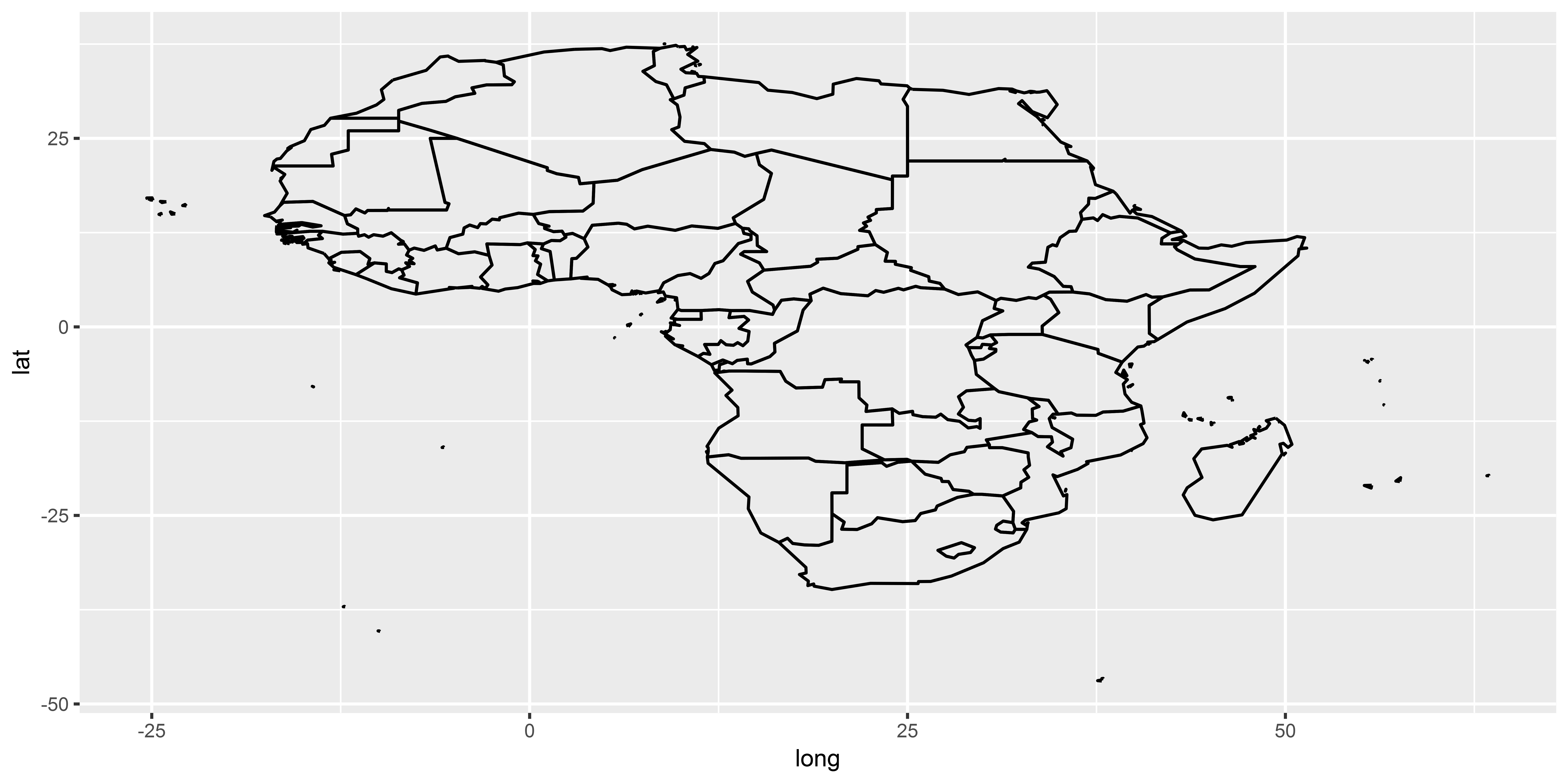
Plot the map! (continued)
africa_map <- ggplot() +
  geom_path(data = africa_fort,
            aes(x = long, y = lat, group = group),
            color = "black")  +
  geom_map(data = africa_fort,
           aes(map_id = id,
               fill = lifeExp),
           map = africa_fort)

plot(africa_map)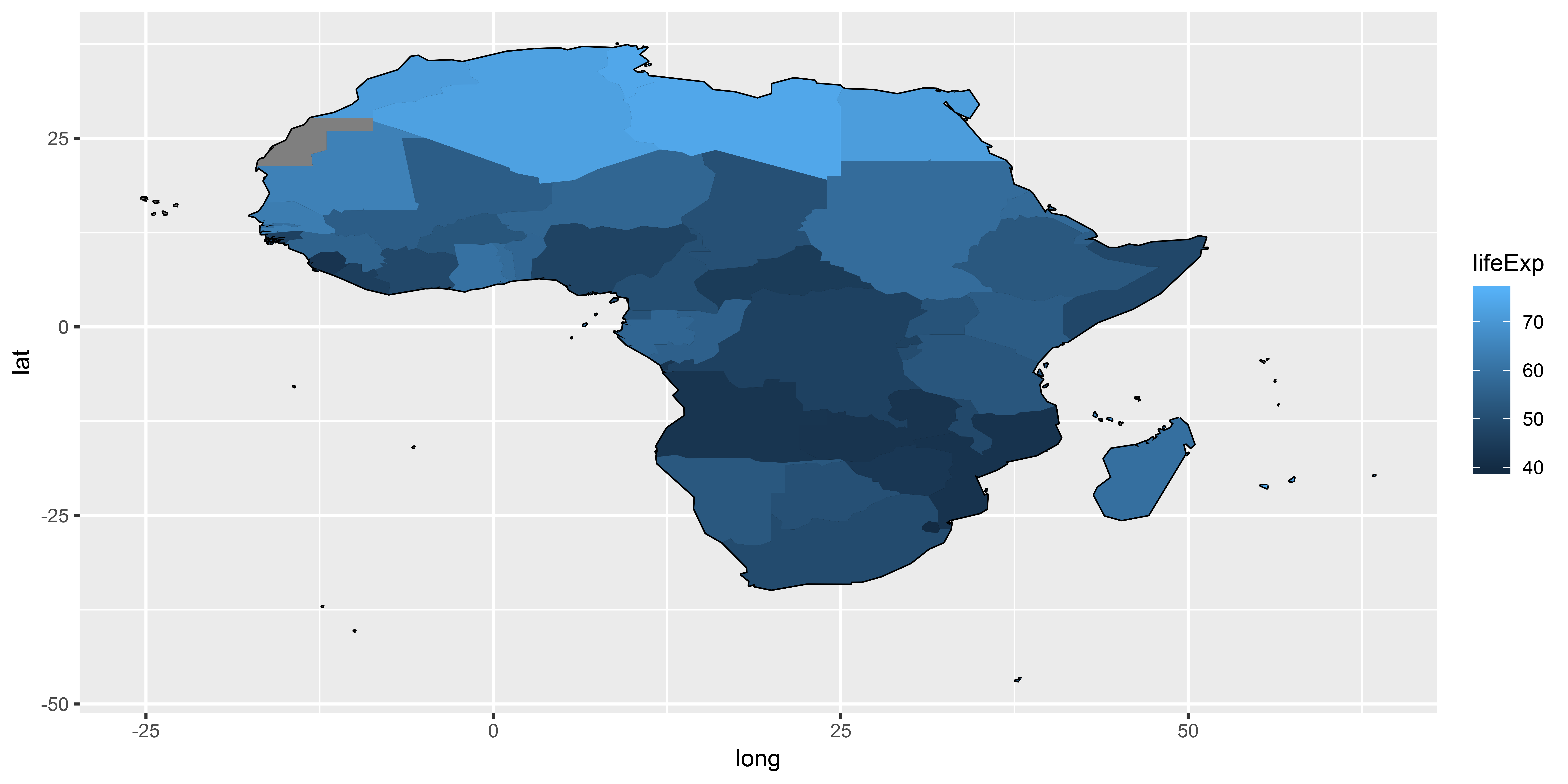
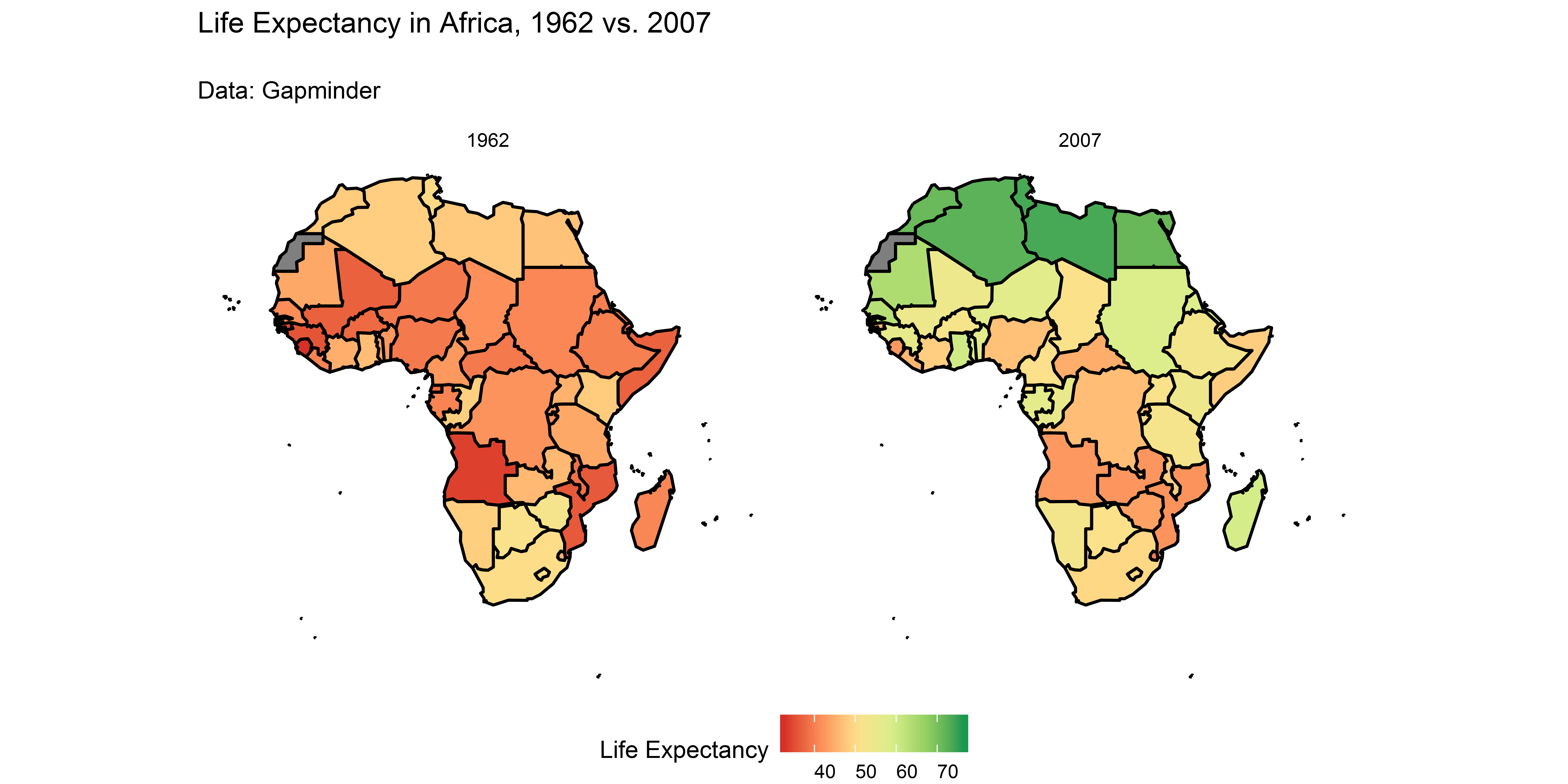
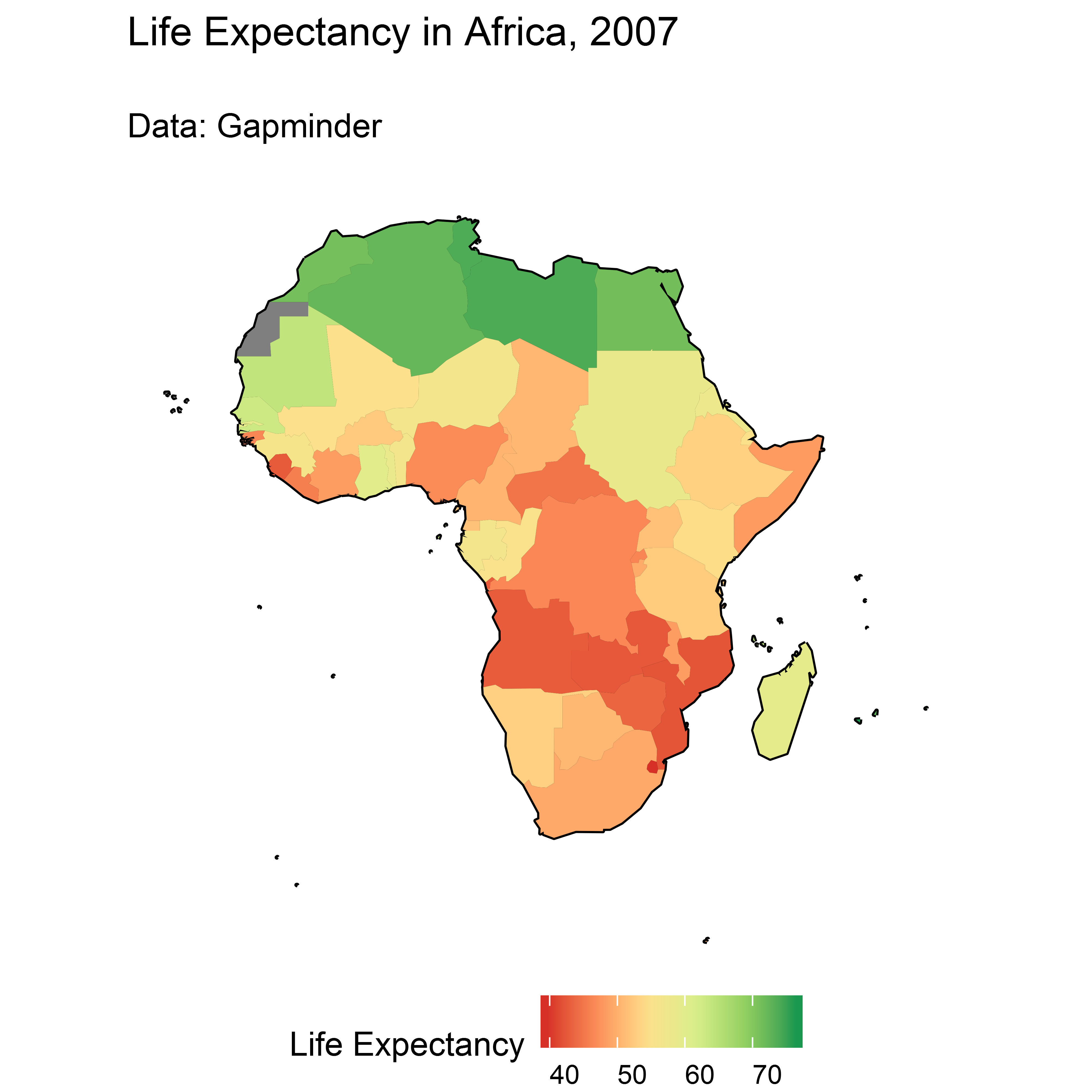
Plot the map! (continued)
africa_map <- ggplot() +
  geom_path(data = africa_fort,
            aes(x = long, y = lat,
                group = group),
            color = "black")  +
  geom_map(data = africa_fort,
           aes(map_id = id,
               fill = lifeExp),
           map = africa_fort) +

  # appearance
  labs(title = "Life Expectancy in Africa, 2007\n",
       subtitle = "Data: Gapminder\n") +
  scale_fill_distiller("Life Expectancy",
                       palette = "RdYlGn",
                       direction = 1) +
  coord_equal() +
  theme_void() +
  theme(panel.grid = element_blank(),
        legend.position = "bottom",
        legend.text.align = 0)
Plot the map! (continued)
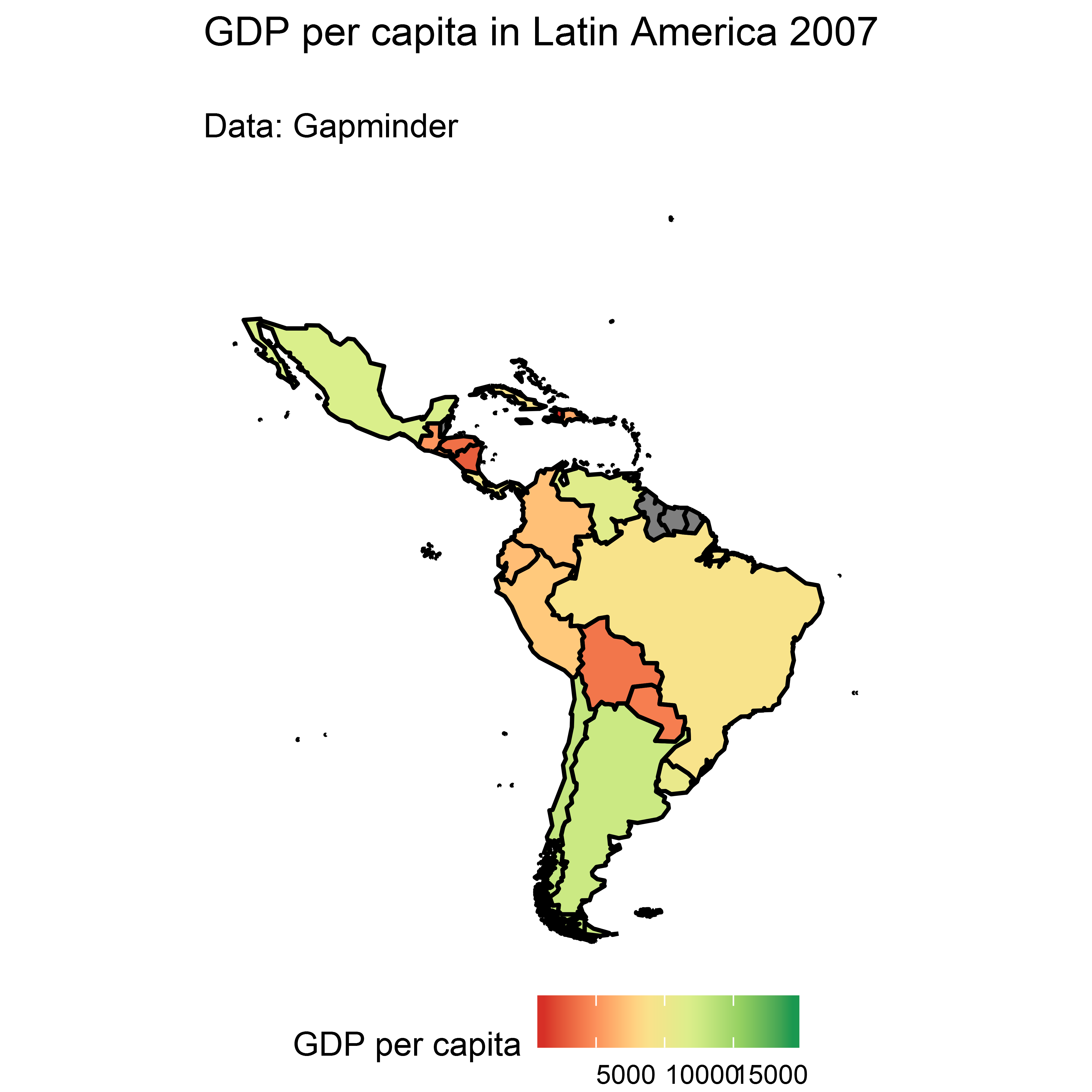
Exercise
Build a map of
Latin America (hint: countrycode has only “Americas” as continent. How would you filter the world shapefile to leave out the US and Canada?)
Merge in information on GDP per capita in 2007
Plot the map
- For the fast ones:
- Read up on the World Development Indicators R package
install.packages(WDI). - Use the package to download data on the indicator
DT.ODA.ODAT.GN.ZS(net development assistance received as percent of GNI) in the year 2015 and download it in a separate data frame Merge the data frame into the
africashapefile and generate a map of Aid/GNI for africa
Solution
library(maptools)
library(sp)
library(countrycode)
library(gapminder)
library(tidyverse)
library(broom)

world <- readShapeSpatial("./data/shapefiles//TM_WORLD_BORDERS_SIMPL-0.3.shp")

world$continent <- countrycode(world$ISO2, "iso2c", "continent")

latam <- subset(world, continent == "Americas")

# remove US and Canada and Greenland
latam <- subset(latam, NAME != "United States" &
                  NAME != "Canada" &
                  NAME != "Greenland")

# get gapminder data
data("gapminder")

gapminder$ISO3 <- countrycode(gapminder$country, "country.name", "iso3c")

gapminder2007 <- gapminder[gapminder$year == 2007, ]
Solution II
# Prepare and Merge Data

latam_fort <- tidy(latam, region = "ISO3")
latam_fort <- left_join(latam_fort,
                         gapminder2007,
                         by = c("id" = "ISO3"))
# plot
latam_map <- ggplot() +
  geom_map(data = latam_fort,
           aes(map_id = id, fill = gdpPercap),
           map = latam_fort) +
  geom_path(data = latam_fort,
            aes(x = long, y = lat, group = group),
            color = "black") +
  labs(title = "GDP per capita in Latin America 2007\n",
       subtitle = "Data: Gapminder\n") +
  scale_fill_distiller("GDP per capita",
                       palette = "RdYlGn",
                       direction = 1) +
  coord_equal() +
  theme_void() +
  theme(panel.grid = element_blank(), legend.position = "bottom",
        legend.text.align = 0)
Solution III