Main steps for building an app
- Set main goal for the app
- Install R Studio and necessary packages (e.g. shiny)
- Select visualization
- Prepare the data accordignly
- Code the app
- Deploy and share the app
Pau Palop-Garcia
GIGA Hamburg and Freie Universität zu Berlin
Research interests: migration, political transnationalism, representation
| Time | Topic |
|---|---|
| 10.00-10.30 | Session 1: Introduction and main goals |
| 10.30-12.00 | Session 2: Basics for building an app |
| 12.00-13.00 | Lunch break |
| 13.00-14.00 | Session 3: Examples I - Scatter plots- |
| 14.00-14.15 | Coffee break |
| 14.15-15.30 | Session 4: Examples II - Interactive maps- |
| 15.30-16.00 | Session 5: Deploying and sharing apps |
Falta 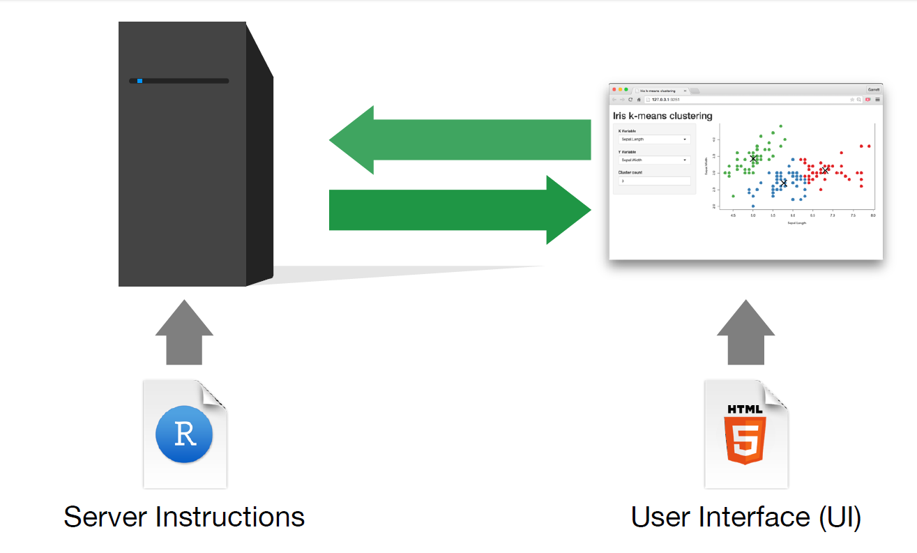
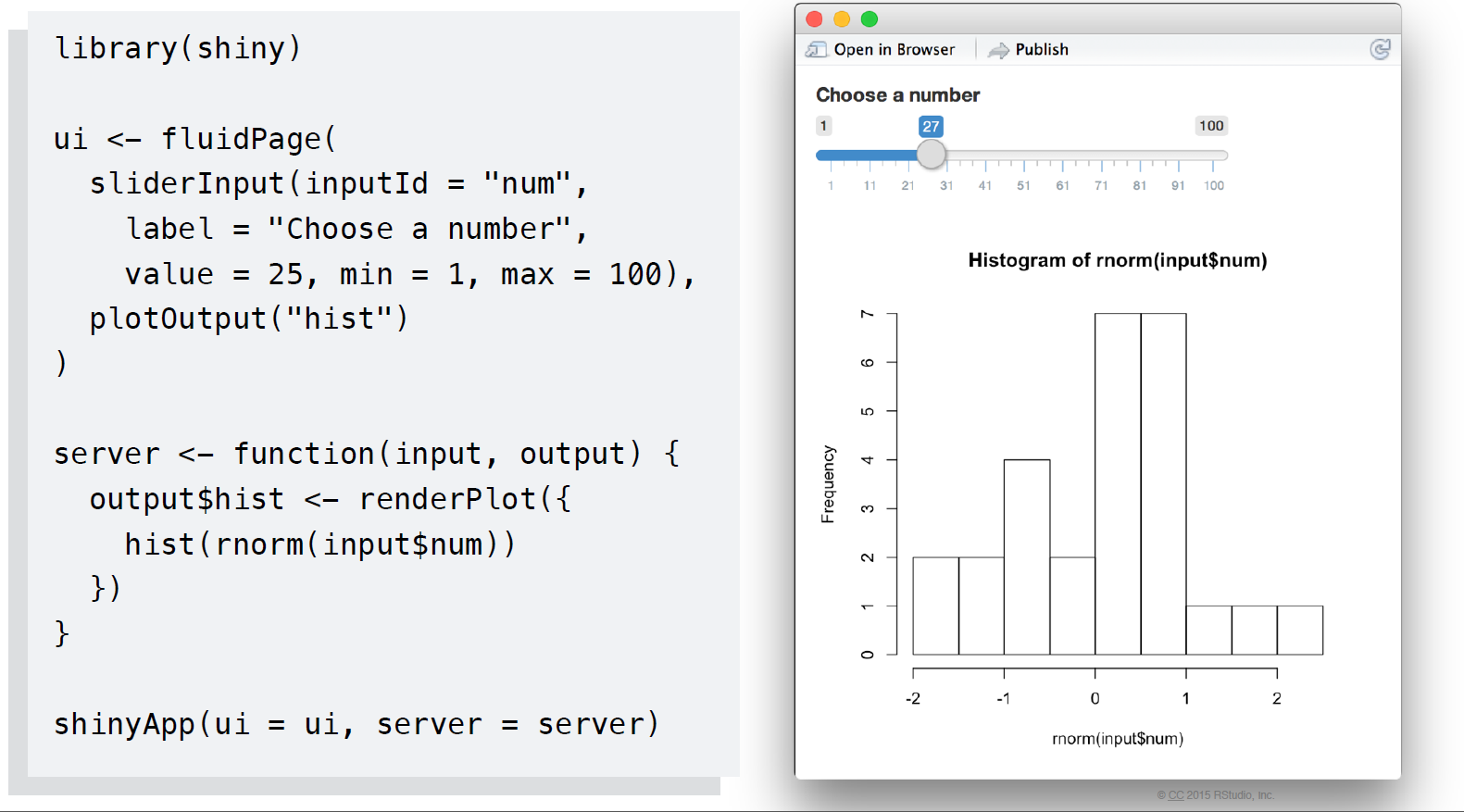
Source: CC 2015, RStudio, Inc
## Warning: package 'shiny' was built under R version 3.4.4## PhantomJS not found. You can install it with webshot::install_phantomjs(). If it is installed, please make sure the phantomjs executable can be found via the PATH variable.Source: https://shiny.rstudio.com/gallery/kmeans-example.html
Source: https://shiny.rstudio.com/gallery/telephones-by-region.html
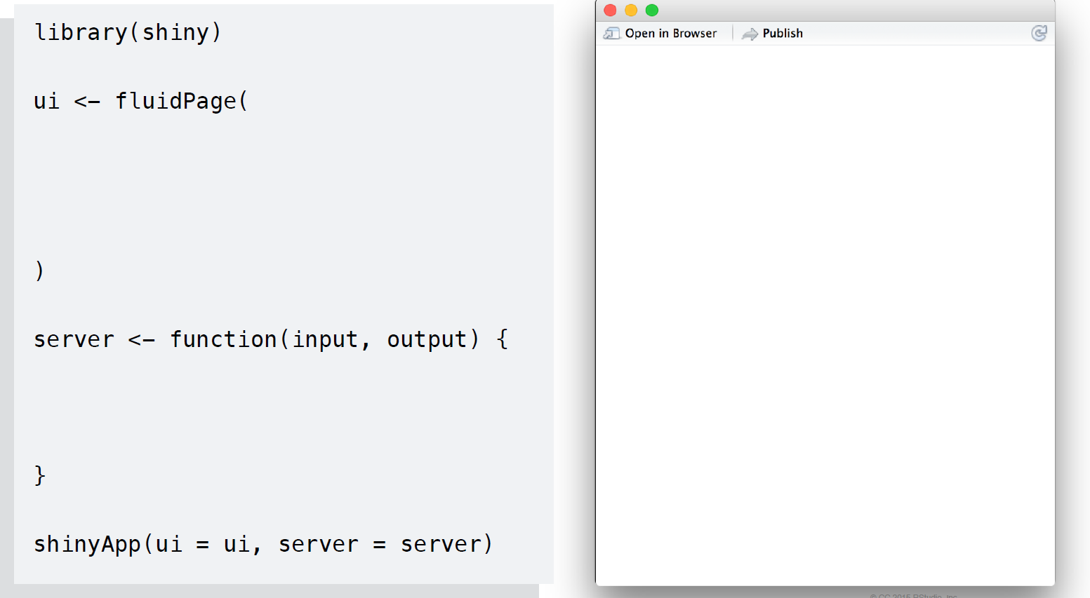
Source: CC 2015 RStudio, Inc
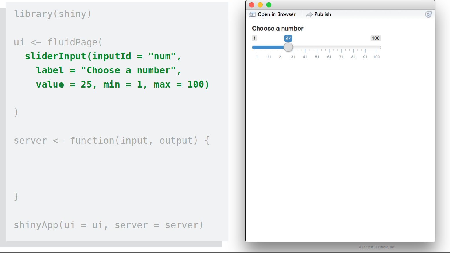
Source: CC 2015 RStudio, Inc
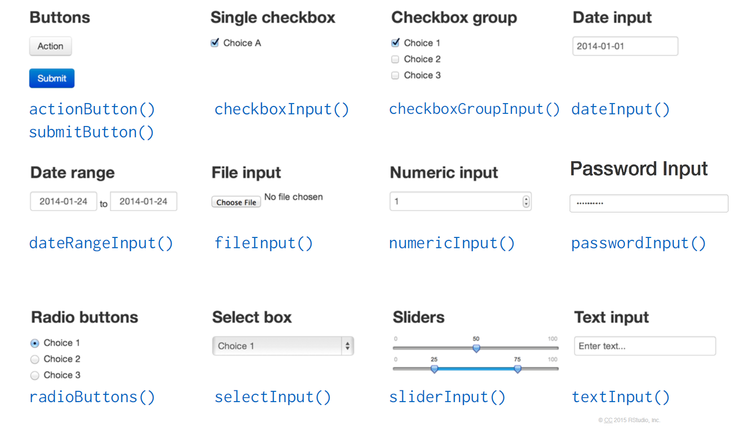
Source: CC 2015 RStudio, Inc
Source: CC 2015 RStudio, Inc
Source: CC 2015 RStudio, Inc
Source: CC 2015 RStudio, Inc
Source: CC 2015, RStudio, Inc
Source: CC 2015 RStudio, Inc
Source: CC 2015 RStudio, Inc
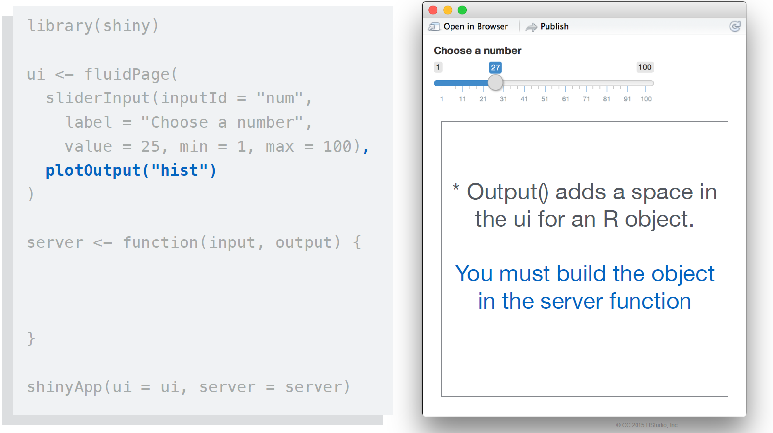
Reactive outputs respond when users toggles a widget
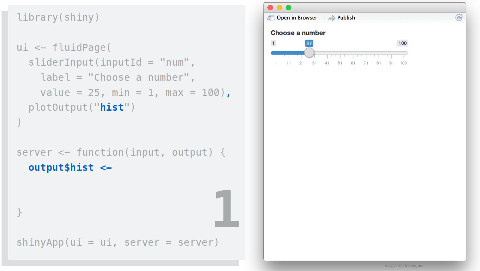
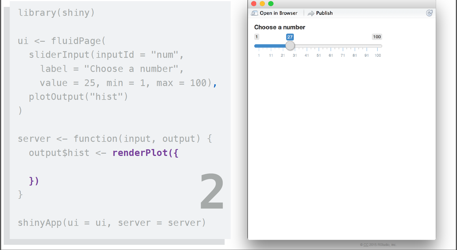
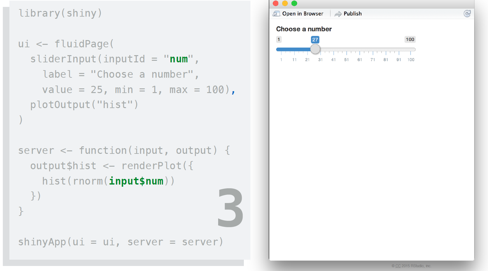
Two main steps: * Add an R object to the user interface * Tell shiny how to build the object in the server function
Source: CC 2015 RStudio, Inc
We will use as a baseline the plot that we created in Session 2 of Day 1. Remmember?
library(gapminder)
library(tidyverse)

example_plot <- ggplot(data = gapminder,
                       # the aes() function defines aesthetics
                       aes(x = year,  # x axis
                           y = lifeExp, # y axis
                           color = continent, # map color to continent
                           size = gdpPercap)) + # map the aesthetic 'size' to gdp/pc
geom_point() library(gapminder)
library(tidyverse)
library(shiny)
ui <- fluidPage(
selectInput("continent", "Select continent",
choices = list("Africa", "Americas", "Asia", "Europe", "Oceania")),
plotOutput("gpoint")
)
server <- function(input, output) {
output$gpoint <- renderPlot({
ggplot(data = subset(gapminder, continent == input$continent, select = c(country:gdpPercap)),
# the aes() function defines aesthetics
aes(x = year, # x axis
y = lifeExp, # y axis
color = continent, # map color to continent
size = gdpPercap)) + # map the aesthetic 'size' to gdp/pc
geom_point()
})
}
shinyApp(ui = ui, server = server, options = list(height = 500))library(gapminder)
library(tidyverse)
library(shiny)
ui <- fluidPage(
checkboxGroupInput("continent", "Select continent",
choices = list("Africa", "Americas", "Asia", "Europe", "Oceania"),
selected = "Africa"),
plotOutput("gpoint")
)
server <- function(input, output) {
output$gpoint <- renderPlot({
ggplot(data = subset(gapminder, continent %in% input$continent, select = c(country:gdpPercap)),
# the aes() function defines aesthetics
aes(x = year, # x axis
y = lifeExp, # y axis
color = continent, # map color to continent
size = gdpPercap)) + # map the aesthetic 'size' to gdp/pc
geom_point()
})
}
shinyApp(ui = ui, server = server, options = list(height = 600))library(gapminder)
library(tidyverse)
library(shiny)
ui <- fluidPage(
checkboxGroupInput("continent", "Select continent",
choices = list("Africa", "Americas", "Asia", "Europe", "Oceania"),
selected = "Africa"),
sliderInput("slider", label = h3("GDP per capita"), min = 240,
max = 113600, value = 250),
plotOutput("gpoint")
)
server <- function(input, output) {
output$gpoint <- renderPlot({
ggplot(data = subset(gapminder, continent %in% input$continent &
gdpPercap < input$slider , select = c(country:gdpPercap)),
# the aes() function defines aesthetics
aes(x = year, # x axis
y = lifeExp, # y axis
color = continent, # map color to continent
size = gdpPercap)) + # map the aesthetic 'size' to gdp/pc
geom_point()
})
}
shinyApp(ui = ui, server = server, options = list(height = 700))library(countrycode)
library(maptools)
library(ggplot2)
library(tidyverse)
library(gapminder)
world <- readShapeSpatial("./data/shapefiles/TM_WORLD_BORDERS_SIMPL-0.3.shp")
world$continent <- countrycode(world$ISO3,
"iso3c", # input format
"continent") # output format
africa <- subset(world, continent == "Africa")
# fortify: bring dataset into shape that ggplot can understand
africa_fort <- fortify(africa, # we use the "africa" shapefile from previous slide
region = "ISO3") # this becomes "id" in the fortified dataset
# get gapminder data
data("gapminder")
# create country identifier for merging
gapminder$ISO3 <- countrycode(gapminder$country, "country.name", "iso3c")
#only year 2007
gapminder2007 <- gapminder[gapminder$year == 2007, ]
# join in gapminder data
africa_fort <- left_join(africa_fort,
gapminder2007,
by = c("id" = "ISO3"))
africa_map <- ggplot() +
geom_path(data = africa_fort,
aes(x = long, y = lat,
group = group),
color = "black") +
geom_map(data = africa_fort,
aes(map_id = id,
fill = lifeExp),
map = africa_fort) +
# appearance
labs(title = "Life Expectancy in Africa, 2007\n",
subtitle = "Data: Gapminder\n") +
scale_fill_distiller("Life Expectancy",
palette = "RdYlGn",
direction = 1) +
coord_equal() +
theme_void() +
theme(panel.grid = element_blank(),
legend.position = "bottom",
legend.text.align = 0)
plot(africa_map)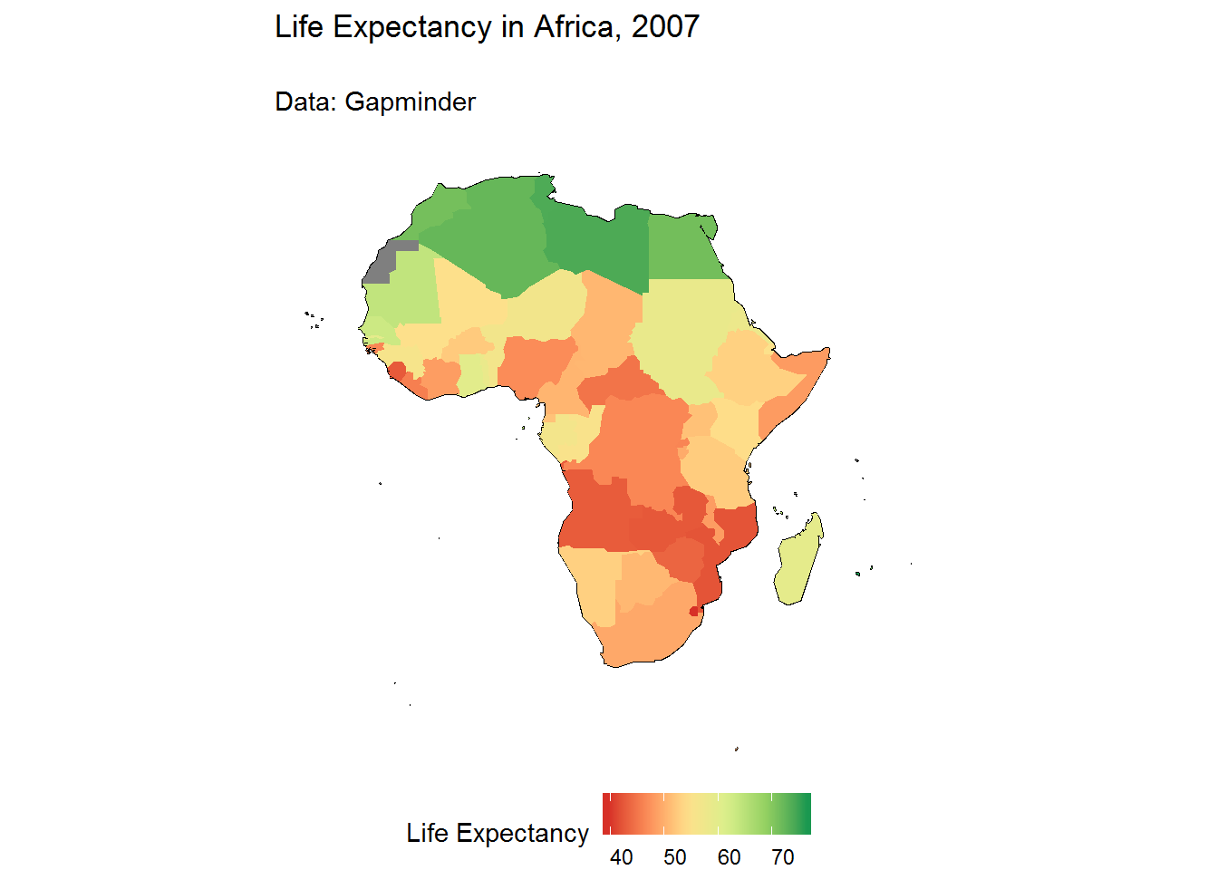
library(countrycode)
library(maptools)
library(ggplot2)
library(tidyverse)
library(gapminder)

ui <- fluidPage(
  radioButtons("variable", "Select variable",
                     choices = list("lifeExp", "pop", "gdpPercap"),
               selected = "lifeExp"),

  plotOutput("gmap")
)


server <- function(input, output) {
  output$gmap <- renderPlot({
    world <- readShapeSpatial("./data/shapefiles/TM_WORLD_BORDERS_SIMPL-0.3.shp")

    world$continent <- countrycode(world$ISO3,
                                   "iso3c", # input format
                                   "continent") # output format

    africa <- subset(world, continent == "Africa")

    # fortify: bring dataset into shape that ggplot can understand
    africa_fort <- fortify(africa, # we use the "africa" shapefile from previous slide
                           region = "ISO3") # this becomes "id" in the fortified dataset


    # get gapminder data
    data("gapminder")

    # create country identifier for merging
    gapminder$ISO3 <- countrycode(gapminder$country, "country.name", "iso3c")

    #only year 2007
    gapminder2007 <- gapminder[gapminder$year == 2007, ]

    # join in gapminder data
    africa_fort <- left_join(africa_fort,
                             gapminder2007,
                             by = c("id" = "ISO3"))

    #Create reactive variable
    africa_fort$var <- africa_fort[,input$variable]

    africa_map <- ggplot() +
      geom_path(data = africa_fort,
                aes(x = long, y = lat,
                    group = group),
                color = "black")  +
      geom_map(data = africa_fort,
               aes(map_id = id,
                   fill = var),
               map = africa_fort) +

      # appearance
      labs(title = "",
           subtitle = "") +
      scale_fill_distiller("",
                           palette = "RdYlGn",
                           direction = 1) +
      coord_equal() +
      theme_void() +
      theme(panel.grid = element_blank(),
            legend.position = "bottom",
            legend.text.align = 0)

    plot(africa_map)
  })
}

shinyApp(ui = ui, server = server, options = list(height = 700))Plot an interactive vizualization in which not only the user can select the variable AND the year that should be plotted. The app layout should include also a sidebar and a mainpanel. Steps:
ui <- pageWithSidebar(
  headerPanel("Select options"),
  sidebarPanel(
    radioButtons("variable", "Select variable",
                 choices = list("Life expectancy" = "lifeExp", "Population" = "pop",
                                "GDP per capita" = "gdpPercap"),
                 selected = "lifeExp"),
    radioButtons("year", label = "Select year",
                 choices = list("1952", "1957", "1962", "1967",
                                "1972", "1977", "1982", "1987",
                                "1992", "1997", "2002", "2007"),
                 selected = "1952")
  ),
  mainPanel(
    plotOutput("gmap")
  )
)


server <- function(input, output) {
  output$gmap <- renderPlot({
    world <- readShapeSpatial("./data/shapefiles/TM_WORLD_BORDERS_SIMPL-0.3.shp")

    world$continent <- countrycode(world$ISO3,
                                   "iso3c", # input format
                                   "continent") # output format

    africa <- subset(world, continent == "Africa")

    # fortify: bring dataset into shape that ggplot can understand
    africa_fort <- fortify(africa, # we use the "africa" shapefile from previous slide
                           region = "ISO3") # this becomes "id" in the fortified dataset


    # get gapminder data
    data("gapminder")

    # create country identifier for merging
    gapminder$ISO3 <- countrycode(gapminder$country, "country.name", "iso3c")

    #only year
    gapminder_year <- gapminder[gapminder$year == input$year, ]

    # join in gapminder data
    africa_fort <- left_join(africa_fort,
                             gapminder_year,
                             by = c("id" = "ISO3"))

    #Create reactive variable
    africa_fort$var <- africa_fort[,input$variable]

    africa_map <- ggplot() +
      geom_path(data = africa_fort,
                aes(x = long, y = lat,
                    group = group),
                color = "gray")  +
      geom_map(data = africa_fort,
               aes(map_id = id,
                   fill = var),
               map = africa_fort) +

      # appearance
      labs(title = "",
           subtitle = "") +
      scale_fill_distiller("",
                           palette = "RdYlGn",
                           direction = 1) +
      coord_equal() +
      theme_void() +
      theme(panel.grid = element_blank(),
            legend.position = "bottom",
            legend.text.align = 0)

    plot(africa_map)
  })
}

shinyApp(ui = ui, server = server, options = list(height = 700))Every shiny app is maintained by a computer running R
How to save it:
Using shinyapps.io:
GIGA 2018