Appendix: Chapter 8 (Public Goods)
Figure E.1: Individual Effects (Corruption)
# Libraries
library(tidyverse)
library(cowplot)
library(lfe)
library(tikzDevice)

# Data
load("./data/diss_df.rda")


# generate cabinetINC label variable for plotting
diss_df$cabinetINClabel <- ifelse(diss_df$cabinetINC == 1, "Power-Sharing",
                                    "No Power-Sharing")

plot_ps_corruption <- ggplot(diss_df, aes(x = cabinetINClabel, y = v2x_corr_t1)) +
  geom_jitter(size = 1.5, alpha = 0.5) +
  geom_boxplot(aes(fill = cabinetINClabel), alpha = 0.6) +
  scale_fill_brewer(palette = "Blues") +
  stat_summary(aes(group = 1), fun.y = mean, geom = "point", shape = 23,
               size = 4, fill = "#d7191c", color = "#d7191c") +
  theme_bw() +
  theme(legend.position = "none", axis.text = element_text(size = 11)) +
  labs(x = "", y = "Political Corruption")


plot_allaid_corruption <- ggplot(diss_df,
                               aes(x = log(aiddata_AidGDP),
                                   y = v2x_corr_t1)) +
  geom_point(alpha = 0.5) +
  geom_smooth(method = "lm") +
  theme_bw() +
  labs(x = "All Aid / GDP (log)",
       y = "Political Corruption")


# Output for Manuscript
# options( tikzDocumentDeclaration = "\\documentclass[11pt]{article}" )
# tikz("../figures/aid_ps_individ_corruption.tex", height = 3.5)
# gridExtra::grid.arrange(plot_ps_corruption, plot_allaid_corruption, nrow = 1)
# dev.off()

# Output for Rep. Archive
gridExtra::grid.arrange(plot_ps_corruption, plot_allaid_corruption, nrow = 1)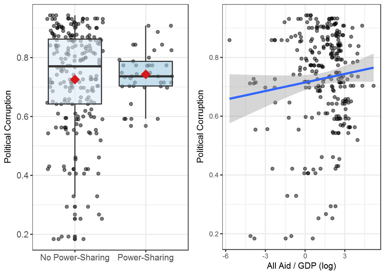
Figure E.2: Model Predictions for the Effect of Foreign Aid and Power-Sharing on
Post-Conflict Particularistic vs. Public Spending
# Libraries
library(tidyverse)
library(rms)
library(gridExtra)
library(tikzDevice)

# Load data
load("data/diss_df.rda")

# to predict substantive effects from this model, we need to define data
# distribution
diss_df$conflictID <- NULL
datadist_diss_df <- datadist(diss_df); options(datadist='datadist_diss_df')

# replicate Model from above with spending + cabCOUNT

model_aidps_spending <- ols(v2dlencmps_t1 ~
                              cabinetCOUNT *
                              aiddata_AidGDP_ln +
                              ln_gdp_pc +
                              ln_pop +
                              conf_intens +
                              nonstate +
                              WBnatres +
                              fh,
                            data=diss_df, x=T, y=T)
model_aidps_spending <- rms::robcov(model_aidps_spending, diss_df$GWNo)

# Start predictions for aid
prediction_democ_aid <- Predict(model_aidps_spending,
                           cabinetCOUNT = c(0, 10), # no / much power-sharing
                           aiddata_AidGDP_ln = seq(-5.7, 5.17, 0.1),# range of aid
                           conf.int = 0.9)

subs_effects_spending_aid <- ggplot(data.frame(prediction_democ_aid),
                                    aes(x = aiddata_AidGDP_ln,
                                        y = yhat,
                                        group = as.factor(cabinetCOUNT))) +
  geom_line( color = "black", size = 1) +
  geom_ribbon(aes(ymax = upper,
                  ymin = lower,
                  fill = as.factor(cabinetCOUNT)),
              alpha = 0.7) +
  scale_fill_manual(values = c("#b3cde3", "#e41a1c"),
                    name = "Number of Rebels \nin the Power-Sharing Coalition:") +
  theme_bw() +
  theme(text = element_text(size=8)) +
  labs(x = "Aid / GDP",
       y = "Predicted Public vs. Particularistic Spending Values") +
  theme(legend.position = "bottom")

# Predictions power-sharing
prediction_democ_ps <- Predict(model_aidps_spending,
                              cabinetCOUNT = seq(0, 10, 1),
                              aiddata_AidGDP_ln = c(0, 3.4),
                              conf.int = 0.9)

prediction_democ_ps$aiddata_AidGDP_ln <- round(exp(prediction_democ_ps$aiddata_AidGDP_ln))


subs_effects_spending_ps <- ggplot(data.frame(prediction_democ_ps),
                                           aes(x = cabinetCOUNT,
                                               y = yhat,
                                               group = as.factor(aiddata_AidGDP_ln))) +
  geom_line( color = "black", size = 1) +
  geom_ribbon(aes(ymax = upper,
                  ymin = lower,
                  fill = as.factor(aiddata_AidGDP_ln)),
              alpha = 0.7) +
  scale_fill_manual(values = c("#b3cde3", "#e41a1c"),
                    name = "Aid in per cent of GDP:") +
  theme_bw() +
  scale_x_continuous(breaks = seq(0, 10, 2)) +
  theme(text = element_text(size=8)) +
  labs(x = "Power-Sharing (No. of rebel seats in government)",
       y = "Predicted Public vs. Particularistic Spending Values") +
  theme(legend.position = "bottom")

# output prediction plots


# output plot for predicted VDEM election quality variables


# options( tikzDocumentDeclaration = "\\documentclass[11pt]{article}" )
# tikz("../figures/aidps_spending.tex", height = 4.5, width = 6.5)
# grid.arrange(subs_effects_spending_ps,
#              subs_effects_spending_aid,
#              nrow = 1)
# dev.off()

grid.arrange(subs_effects_spending_ps,
             subs_effects_spending_aid,
             nrow = 1)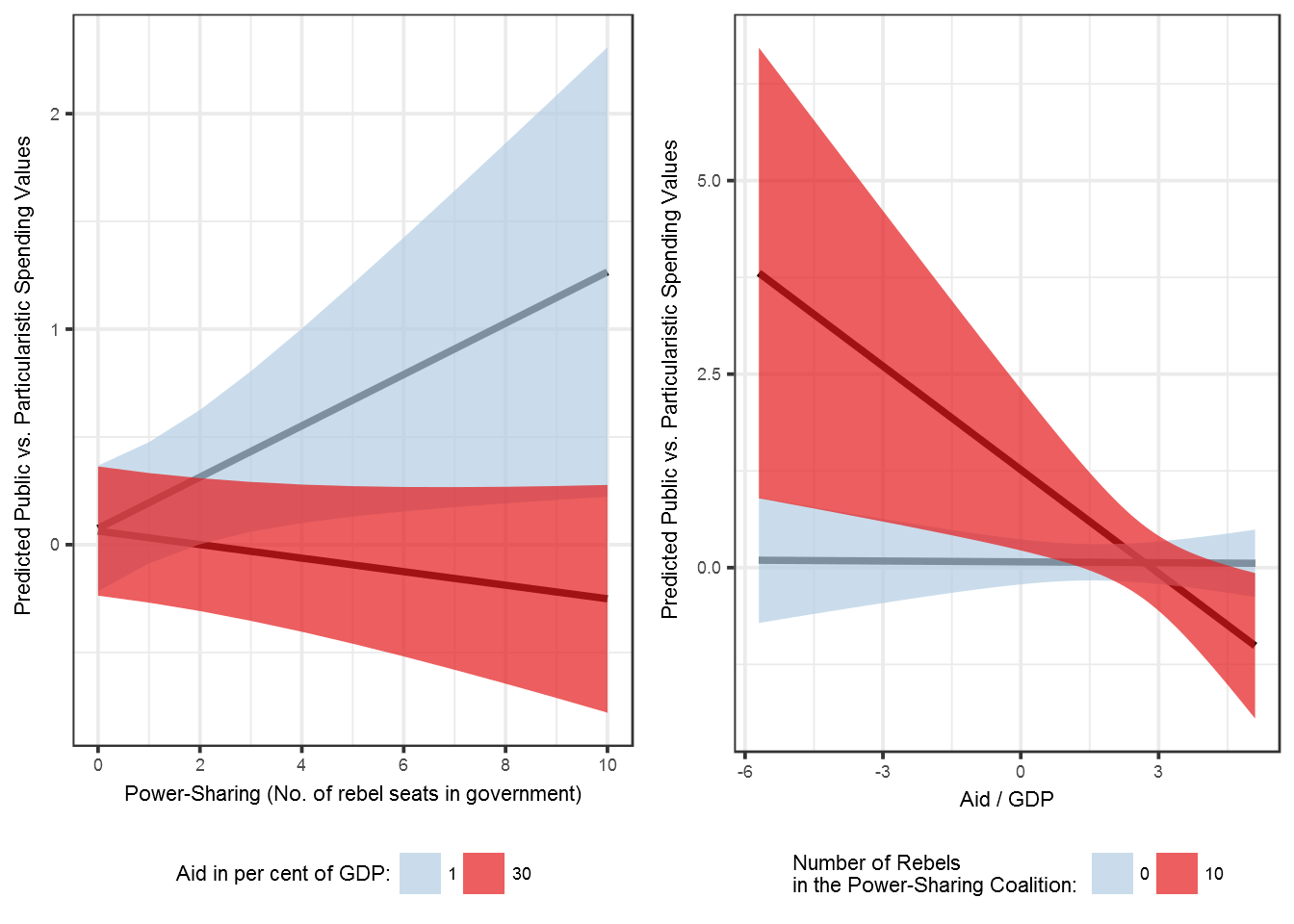
Table E.1: Power-Sharing, Foreign Aid, and Post-Conflict Provision of Public
Goods: Individual Effects (Corruption as DV)
# Libraries
library(texreg)
source("functions/extract_ols_custom.R")
library(rms)


# load Data
load("./data/diss_df.rda")

# Power-Sharing Models
model_ps_corruption_cabcount <- ols(v2x_corr_t1 ~
                                     cabinetCOUNT +
                                     aiddata_AidGDP_ln +
                                     ln_gdp_pc +
                                     ln_pop +
                                     conf_intens +
                                     nonstate +
                                     WBnatres +
                                     fh,
                                   data=diss_df, x=T, y=T)
model_ps_corruption_cabcount <- rms::robcov(model_ps_corruption_cabcount, diss_df$GWNo)


model_ps_corruption_seniorcount <- ols(v2x_corr_t1 ~
                              seniorCOUNT  +
                              aiddata_AidGDP_ln +
                              ln_gdp_pc +
                              ln_pop +
                              conf_intens +
                              nonstate +
                              WBnatres +
                              fh,
                            data=diss_df, x=T, y=T)
model_ps_corruption_seniorcount <- rms::robcov(model_ps_corruption_seniorcount, diss_df$GWNo)


model_ps_corruption_nonseniorcount <- ols(v2x_corr_t1 ~
                              nonseniorCOUNT *
                              aiddata_AidGDP_ln +
                              ln_gdp_pc +
                              ln_pop +
                              conf_intens +
                              nonstate +
                              WBnatres +
                              fh,
                            data=diss_df, x=T, y=T)
model_ps_corruption_nonseniorcount <- rms::robcov(model_ps_corruption_nonseniorcount, diss_df$GWNo)

# Aid Models

model_dga_corruption <- ols(v2x_corr_t1 ~
                              cabinetCOUNT +
                            log(dga_gdp_zero + 1) +
                              aiddata_AidGDP_ln +
                              ln_gdp_pc +
                              ln_pop +
                              conf_intens +
                              nonstate +
                              WBnatres +
                              fh,
                            data=diss_df, x=T, y=T)
model_dga_corruption <- rms::robcov(model_dga_corruption, diss_df$GWNo)

model_pga_corruption <- ols(v2x_corr_t1 ~
                              cabinetCOUNT +
                            log(program_aid_gdp_zero + 1) +
                              aiddata_AidGDP_ln +
                              ln_gdp_pc +
                              ln_pop +
                              conf_intens +
                              nonstate +
                              WBnatres +
                              fh,
                            data=diss_df, x=T, y=T)
model_pga_corruption <- rms::robcov(model_pga_corruption, diss_df$GWNo)

model_bga_corruption <- ols(v2x_corr_t1 ~
                              cabinetCOUNT +
                            log(commodity_aid_gdp_zero + 1) +
                              aiddata_AidGDP_ln +
                              ln_gdp_pc +
                              ln_pop +
                              conf_intens +
                              nonstate +
                              WBnatres +
                              fh,
                            data=diss_df, x=T, y=T)
model_bga_corruption <- rms::robcov(model_bga_corruption, diss_df$GWNo)


model_list <- list(model_ps_corruption_cabcount,
                   model_ps_corruption_seniorcount,
                   model_ps_corruption_nonseniorcount,
                   model_dga_corruption,
                   model_pga_corruption,
                   model_bga_corruption)

coef_name_map <- list(
                      cabinetINC = "Power-Sharing (binary)",
                      "cabinetINC * aiddata_AidGDP_ln" = "Power-Sharing (binary) * Aid",
                      cabinetCOUNT = "Power-Sharing (cabinet)",
                                            seniorCOUNT = "Power-Sharing (senior)",
                      nonseniorCOUNT = "Power-Sharing (nonsenior)",

                      "cabinetCOUNT * aiddata_AidGDP_ln" = "Power-Sharing (cabinet) * Aid",
                      "cabinetCOUNT:aiddata_AidGDP_ln" = "PS (cabinet) * Aid",
                      ps_share = "PS (cabinet share)",
                      "ps_share * aiddata_AidGDP_ln" = "PS (cabinet share) * Aid",
                      dga_gdp_zero = "DGA/GDP (log)",
                      program_aid_gdp_zero = "Program Aid/GDP (log)",
                      commodity_aid_gdp_zero = "Budget Aid/GDP (log)",
                      aiddata_AidGDP_ln = "Aid / GDP (log)",

                      ln_gdp_pc = "GDP p/c (log)",
                      ln_pop = "Population (log)",
                      conf_intens = "Conflict Intensity",
                      nonstate = "Non-State Violence",
                      WBnatres = "Nat. Res. Rents",
                      polity2 = "Polity",
                      fh = "Regime Type (FH)",
                      Ethnic = "Ethnic Frac.",
                      DS_ordinal = "UN PKO")

# custom functions to write tex output
source("./functions/custom_texreg.R")
environment(custom_texreg) <- asNamespace('texreg')
#
#
# # Output Manuscript
# custom_texreg(l = model_list,
#           stars = c(0.001, 0.01, 0.05, 0.1),
#           custom.coef.map = coef_name_map,
#        file = "../output/aid_ps_indeff_corr.tex",
#           symbol = "+",
#           table = F,
#           booktabs = T,
#           use.packages = F,
#           dcolumn = T,
#           include.lr = F,
#           include.rsquared = F,
#                  include.cluster = T,
#
#           include.adjrs = T,
#         caption = "",
#               custom.multicol = T,
#               custom.model.names = c(" \\multicolumn{3}{c}{ \\textbf{Power-Sharing}} & \\multicolumn{3}{c}{ \\textbf{Foreign Aid}} \\\\ \\cmidrule(r){2-4} \\cmidrule(l){5-7} & \\multicolumn{1}{c}{(1)  }",
#                                      "\\multicolumn{1}{c}{(2)  }",
#                                      "\\multicolumn{1}{c}{(3)  }",
#                                      "\\multicolumn{1}{c}{(4)  }",
#                                      "\\multicolumn{1}{c}{(5)   }",
#                                      "\\multicolumn{1}{c}{(6)   }"))


# Output Replication Archive
htmlreg(l = model_list,
          stars = c(0.001, 0.01, 0.05, 0.1),
          custom.coef.map = coef_name_map,
          symbol = "+",
          table = F,
          booktabs = T,
          use.packages = F,

          dcolumn = T,
          include.lr = F,
          include.rsquared = F,
          include.adjrs = T,
          include.cluster = T,
        caption = "",
star.symbol = "\\*")| Model 1 | Model 2 | Model 3 | Model 4 | Model 5 | Model 6 | ||
|---|---|---|---|---|---|---|---|
| Power-Sharing (cabinet) | 0.00 | 0.00 | 0.00 | 0.00 | |||
| (0.00) | (0.00) | (0.00) | (0.00) | ||||
| Power-Sharing (senior) | 0.00 | ||||||
| (0.01) | |||||||
| Power-Sharing (nonsenior) | 0.01 | ||||||
| (0.02) | |||||||
| DGA/GDP (log) | -0.04 | ||||||
| (0.03) | |||||||
| Program Aid/GDP (log) | -0.05* | ||||||
| (0.03) | |||||||
| Budget Aid/GDP (log) | -0.00 | ||||||
| (0.02) | |||||||
| Aid / GDP (log) | -0.00 | -0.00 | -0.00 | 0.00 | 0.01 | -0.00 | |
| (0.01) | (0.01) | (0.01) | (0.01) | (0.01) | (0.02) | ||
| GDP p/c (log) | -0.03 | -0.03 | -0.03 | -0.03 | -0.05+ | -0.03 | |
| (0.02) | (0.02) | (0.02) | (0.02) | (0.03) | (0.02) | ||
| Population (log) | 0.02 | 0.02 | 0.02 | 0.02+ | 0.02 | 0.02 | |
| (0.01) | (0.01) | (0.01) | (0.01) | (0.01) | (0.01) | ||
| Conflict Intensity | -0.04 | -0.04 | -0.04 | -0.03 | -0.03 | -0.04 | |
| (0.03) | (0.03) | (0.03) | (0.04) | (0.03) | (0.03) | ||
| Non-State Violence | 0.03 | 0.03 | 0.03 | 0.02 | 0.02 | 0.03 | |
| (0.03) | (0.03) | (0.03) | (0.03) | (0.03) | (0.03) | ||
| Nat. Res. Rents | 0.00 | 0.00 | 0.00 | 0.00 | 0.00 | 0.00 | |
| (0.00) | (0.00) | (0.00) | (0.00) | (0.00) | (0.00) | ||
| Regime Type (FH) | -0.06*** | -0.06*** | -0.06*** | -0.06*** | -0.06*** | -0.06*** | |
| (0.01) | (0.01) | (0.01) | (0.01) | (0.01) | (0.01) | ||
| Num. obs. | 273 | 273 | 273 | 273 | 273 | 273 | |
| Countries | 46 | 46 | 46 | 46 | 46 | 46 | |
| Adj. R2 | 0.43 | 0.43 | 0.42 | 0.43 | 0.44 | 0.42 | |
| ***p < 0.001, **p < 0.01, *p < 0.05, +p < 0.1 | |||||||
Table E.2: Robustness: Power-Sharing, Foreign Aid, and Public vs. Particularistic Spending (Outliers, Time, Power-Sharing Codings
# Libraries
library(texreg)
source("functions/extract_ols_custom.R")
library(rms)


load("./data/diss_df.rda")

# Outliers
# Load outlier function
source("./functions/outlier_analysis.R")

# Estimate baseline model
model_spending_cabcount <- rms::ols(v2dlencmps_t1 ~
                        cabinetCOUNT *
                        aiddata_AidGDP_ln +
                        log(GDP_per_capita) +
                        log(population) +
                        conf_intens +
                        nonstate +
                        WBnatres +
                        fh ,
                      data=diss_df, x=T, y=T)
model_spending_cabcount <- rms::robcov(model_spending_cabcount, diss_df$GWNo)

# selector variables
selectvars = c("Location", "year", "identifiers")
diss_df$identifiers <- paste(diss_df$GWNo, diss_df$year, sep = "-")

# Estimate outliers
spending_outliers <- check_outlier(model_spending_cabcount,
                                      data = diss_df,
                                      selectvars = selectvars,
                                clustervar = "GWNo")


# Time
model_spending_time <- rms::ols(v2dlencmps_t1 ~
                        cabinetCOUNT *
                        aiddata_AidGDP_ln +
                        log(GDP_per_capita) +
                        log(population) +
                        conf_intens +
                        nonstate +
                        WBnatres +
                        fh +
                          pcy + pcy2 + pcy3,
                      data=diss_df, x=T, y=T)
model_spending_time <- rms::robcov(model_spending_time, diss_df$GWNo)

# year FE
diss_df$yearFE <- as.factor(diss_df$year)
model_spending_yearfe <- rms::ols(v2dlencmps_t1 ~
                        cabinetCOUNT *
                        aiddata_AidGDP_ln +
                        log(GDP_per_capita) +
                        log(population) +
                        conf_intens +
                        nonstate +
                        WBnatres +
                        fh +
                        yearFE,
                      data=diss_df, x=T, y=T)
model_spending_yearfe <- rms::robcov(model_spending_yearfe, diss_df$GWNo)


# different cabinet aggregation types
model_spending_cabmax <- rms::ols(v2dlencmps_t1 ~
                        cabinetCOUNT_max *
                        aiddata_AidGDP_ln +
                        log(GDP_per_capita) +
                        log(population) +
                        conf_intens +
                        nonstate +
                        WBnatres +
                        fh ,
                      data=diss_df, x=T, y=T)
model_spending_cabmax <- rms::robcov(model_spending_cabmax, diss_df$GWNo)

model_spending_cabmin <- rms::ols(v2dlencmps_t1 ~
                        cabinetCOUNT_min *
                        aiddata_AidGDP_ln +
                        log(GDP_per_capita) +
                        log(population) +
                        conf_intens +
                        nonstate +
                        WBnatres +
                        fh ,
                      data=diss_df, x=T, y=T)
model_spending_cabmin <- rms::robcov(model_spending_cabmin, diss_df$GWNo)


model_spending_cabsix <- rms::ols(v2dlencmps_t1 ~
                        cabinetCOUNT_six *
                        aiddata_AidGDP_ln +
                        log(GDP_per_capita) +
                        log(population) +
                        conf_intens +
                        nonstate +
                        WBnatres +
                        fh ,
                      data=diss_df, x=T, y=T)
model_spending_cabsix <- rms::robcov(model_spending_cabsix, diss_df$GWNo)

model_list <- list(spending_outliers[[2]],
          spending_outliers[[4]],
          spending_outliers[[6]],
          model_spending_time,
          model_spending_yearfe,
          model_spending_cabmax,
          model_spending_cabmin,
          model_spending_cabsix)

coef_map <- list(cabinetCOUNT = "Power-Sharing (cabinet)",
                   cabinetCOUNT_max = "Power-Sharing (cabinet)",
                   cabinetCOUNT_min = "Power-Sharing (cabinet)",
                   cabinetCOUNT_six = "Power-Sharing (cabinet)",
                   "cabinetCOUNT * aiddata_AidGDP_ln" = "Power-Sharing (cabinet) * Aid",
                   "cabinetCOUNT_max * aiddata_AidGDP_ln" = "Power-Sharing (cabinet) * Aid",
                   "cabinetCOUNT_min * aiddata_AidGDP_ln" = "Power-Sharing (cabinet) * Aid",
                   "cabinetCOUNT_six * aiddata_AidGDP_ln" = "Power-Sharing (cabinet) * Aid",
                   aiddata_AidGDP_ln = "Aid / GDP (log)",
                   GDP_per_capita = "GDP p/c",
                   population = "Population",
                   conf_intens = "Conflict Intensity",
                   nonstate = "Non-State Violence",
                   WBnatres = "Nat. Res. Rents",
                   polity2 = "Polity",
                 fh = "Regime Type (FH)",
                   pcy = "Time",
                   pcy2 = "Time$^2$",
                   pcy3 = "Time$^3$")
#
# texreg::texreg(model_list,
#        stars = c(0.001, 0.01, 0.05, 0.1),
#        custom.coef.map = coef_map,
#        file = "../output/aidps_spending_tech_rob.tex",
#        symbol = "+",
#        table = F,
#        booktabs = T,
#        use.packages = F,
#        dcolumn = T,
#        include.lr = F,
#        custom.model.names = c("(1) Hat Values",
#                               "(2) Cook's Distance",
#                               "(3) DFBETA",
#
#                               "(4) Cubic Time Trend",
#                                "(5) Year FE",
#                                "(6) PS: Max",
#                                "(7) PS: Min",
#                                "(8) PS: Six Months"),
#        include.adjrs = T,
#        caption = "",
#        star.symbol = "\\*",
#        include.rsquared = F,
#        include.cluster = T,
#        include.variance = F)

# Output Replication Archive
htmlreg(model_list,
                stars = c(0.001, 0.01, 0.05, 0.1),
                custom.coef.map = coef_map,
                symbol = "+",
                table = F,
                booktabs = T,
                use.packages = F,
                dcolumn = T,
                 custom.model.names = c("(1) Hat Values",
                              "(2) Cook's Distance",
                              "(3) DFBETA",

                              "(2) Cubic Time Trend",
                               "(3) Year FE",
                               "(4) PS: Max",
                               "(5) PS: Min",
                               "(6) PS: Six Months"),
                include.lr = F,
                include.adjrs = T,
                caption = "",
                star.symbol = "\\*",
                include.rsquared = F,
                include.cluster = T,
include.variance = F)| (1) Hat Values | (2) Cook’s Distance | (3) DFBETA | (2) Cubic Time Trend | (3) Year FE | (4) PS: Max | (5) PS: Min | (6) PS: Six Months | ||
|---|---|---|---|---|---|---|---|---|---|
| Power-Sharing (cabinet) | 0.63** | 0.13+ | 0.31*** | 0.12+ | 0.10 | 0.13** | 0.11 | 0.11 | |
| (0.22) | (0.08) | (0.08) | (0.07) | (0.07) | (0.05) | (0.08) | (0.07) | ||
| Power-Sharing (cabinet) * Aid | -0.24* | -0.05* | -0.12*** | -0.04* | -0.04+ | -0.04** | -0.05+ | -0.04* | |
| (0.11) | (0.02) | (0.03) | (0.02) | (0.02) | (0.01) | (0.03) | (0.02) | ||
| Aid / GDP (log) | 0.00 | -0.03 | -0.01 | -0.00 | -0.02 | -0.01 | -0.00 | -0.00 | |
| (0.08) | (0.05) | (0.04) | (0.07) | (0.07) | (0.06) | (0.06) | (0.06) | ||
| GDP p/c | -0.35** | -0.40*** | -0.42*** | -0.37*** | -0.39** | -0.37*** | -0.36*** | -0.36*** | |
| (0.12) | (0.10) | (0.08) | (0.11) | (0.12) | (0.11) | (0.11) | (0.11) | ||
| Population | 0.08 | 0.07 | 0.07 | 0.06 | 0.04 | 0.06 | 0.06 | 0.06 | |
| (0.10) | (0.08) | (0.05) | (0.09) | (0.09) | (0.09) | (0.09) | (0.09) | ||
| Conflict Intensity | 0.16 | 0.25 | 0.22 | 0.11 | 0.11 | 0.10 | 0.11 | 0.11 | |
| (0.22) | (0.21) | (0.17) | (0.22) | (0.21) | (0.22) | (0.22) | (0.22) | ||
| Non-State Violence | -1.05* | -0.68** | -0.88*** | -0.91* | -0.89* | -0.92* | -0.92* | -0.90* | |
| (0.44) | (0.22) | (0.27) | (0.40) | (0.41) | (0.40) | (0.40) | (0.41) | ||
| Nat. Res. Rents | -0.01 | -0.01* | -0.01+ | -0.00 | -0.00 | -0.00 | -0.00 | -0.00 | |
| (0.01) | (0.00) | (0.00) | (0.01) | (0.01) | (0.01) | (0.01) | (0.01) | ||
| Regime Type (FH) | 0.39*** | 0.33*** | 0.33*** | 0.40*** | 0.40*** | 0.40*** | 0.39*** | 0.39*** | |
| (0.08) | (0.07) | (0.06) | (0.08) | (0.08) | (0.08) | (0.08) | (0.08) | ||
| Time | -0.37 | ||||||||
| (0.26) | |||||||||
| Time\(^2\) | 0.11 | ||||||||
| (0.09) | |||||||||
| Time\(^3\) | -0.01 | ||||||||
| (0.01) | |||||||||
| Num. obs. | 251 | 260 | 197 | 273 | 273 | 273 | 273 | 273 | |
| Countries | 45 | 45 | 45 | 46 | 46 | 46 | 46 | 46 | |
| Adj. R2 | 0.38 | 0.35 | 0.48 | 0.35 | 0.32 | 0.36 | 0.35 | 0.35 | |
| ***p < 0.001, **p < 0.01, *p < 0.05, +p < 0.1 | |||||||||
LS0tDQp0aXRsZTogIkFwcGVuZGl4OiBDaGFwdGVyIDggKFB1YmxpYyBHb29kcykiDQpvdXRwdXQ6IA0KICBodG1sX2RvY3VtZW50Og0KICAgIHRvYzogdHJ1ZQ0KICAgIHRvY19mbG9hdDogDQogICAgICBjb2xsYXBzZWQ6IGZhbHNlDQogICAgY29kZV9kb3dubG9hZDogdHJ1ZQ0KICAgIGNvZGVfZm9sZGluZzogImhpZGUiDQoNCi0tLQ0KDQoNCiMgRmlndXJlIEUuMTogSW5kaXZpZHVhbCBFZmZlY3RzIChDb3JydXB0aW9uKQ0KDQpgYGB7ciwgZmlnLmFsaWduID0gImNlbnRlciIsIG1lc3NhZ2U9Riwgd2FybmluZz1GLCBjYWNoZSA9IFQsIGNvbW1lbnRzID0gRiwgd2lkdGggPSA5LCBoZWlnaHQgPSA0LCBkZXYgPSAiQ2Fpcm9QTkciIH0NCiMgTGlicmFyaWVzDQpsaWJyYXJ5KHRpZHl2ZXJzZSkNCmxpYnJhcnkoY293cGxvdCkNCmxpYnJhcnkobGZlKQ0KbGlicmFyeSh0aWt6RGV2aWNlKQ0KDQojIERhdGENCmxvYWQoIi4vZGF0YS9kaXNzX2RmLnJkYSIpDQoNCg0KIyBnZW5lcmF0ZSBjYWJpbmV0SU5DIGxhYmVsIHZhcmlhYmxlIGZvciBwbG90dGluZw0KZGlzc19kZiRjYWJpbmV0SU5DbGFiZWwgPC0gaWZlbHNlKGRpc3NfZGYkY2FiaW5ldElOQyA9PSAxLCAiUG93ZXItU2hhcmluZyIsIA0KICAgICAgICAgICAgICAgICAgICAgICAgICAgICAgICAgICAgIk5vIFBvd2VyLVNoYXJpbmciKQ0KDQpwbG90X3BzX2NvcnJ1cHRpb24gPC0gZ2dwbG90KGRpc3NfZGYsIGFlcyh4ID0gY2FiaW5ldElOQ2xhYmVsLCB5ID0gdjJ4X2NvcnJfdDEpKSArIA0KICBnZW9tX2ppdHRlcihzaXplID0gMS41LCBhbHBoYSA9IDAuNSkgKw0KICBnZW9tX2JveHBsb3QoYWVzKGZpbGwgPSBjYWJpbmV0SU5DbGFiZWwpLCBhbHBoYSA9IDAuNikgKw0KICBzY2FsZV9maWxsX2JyZXdlcihwYWxldHRlID0gIkJsdWVzIikgKyANCiAgc3RhdF9zdW1tYXJ5KGFlcyhncm91cCA9IDEpLCBmdW4ueSA9IG1lYW4sIGdlb20gPSAicG9pbnQiLCBzaGFwZSA9IDIzLA0KICAgICAgICAgICAgICAgc2l6ZSA9IDQsIGZpbGwgPSAiI2Q3MTkxYyIsIGNvbG9yID0gIiNkNzE5MWMiKSArIA0KICB0aGVtZV9idygpICsNCiAgdGhlbWUobGVnZW5kLnBvc2l0aW9uID0gIm5vbmUiLCBheGlzLnRleHQgPSBlbGVtZW50X3RleHQoc2l6ZSA9IDExKSkgKw0KICBsYWJzKHggPSAiIiwgeSA9ICJQb2xpdGljYWwgQ29ycnVwdGlvbiIpDQoNCg0KcGxvdF9hbGxhaWRfY29ycnVwdGlvbiA8LSBnZ3Bsb3QoZGlzc19kZiwgDQogICAgICAgICAgICAgICAgICAgICAgICAgICAgICAgYWVzKHggPSBsb2coYWlkZGF0YV9BaWRHRFApLCANCiAgICAgICAgICAgICAgICAgICAgICAgICAgICAgICAgICAgeSA9IHYyeF9jb3JyX3QxKSkgKyANCiAgZ2VvbV9wb2ludChhbHBoYSA9IDAuNSkgKw0KICBnZW9tX3Ntb290aChtZXRob2QgPSAibG0iKSArDQogIHRoZW1lX2J3KCkgKw0KICBsYWJzKHggPSAiQWxsIEFpZCAvIEdEUCAobG9nKSIsIA0KICAgICAgIHkgPSAiUG9saXRpY2FsIENvcnJ1cHRpb24iKSANCg0KDQojIE91dHB1dCBmb3IgTWFudXNjcmlwdA0KIyBvcHRpb25zKCB0aWt6RG9jdW1lbnREZWNsYXJhdGlvbiA9ICJcXGRvY3VtZW50Y2xhc3NbMTFwdF17YXJ0aWNsZX0iICkNCiMgdGlreigiLi4vZmlndXJlcy9haWRfcHNfaW5kaXZpZF9jb3JydXB0aW9uLnRleCIsIGhlaWdodCA9IDMuNSkNCiMgZ3JpZEV4dHJhOjpncmlkLmFycmFuZ2UocGxvdF9wc19jb3JydXB0aW9uLCBwbG90X2FsbGFpZF9jb3JydXB0aW9uLCBucm93ID0gMSkNCiMgZGV2Lm9mZigpDQoNCiMgT3V0cHV0IGZvciBSZXAuIEFyY2hpdmUNCmdyaWRFeHRyYTo6Z3JpZC5hcnJhbmdlKHBsb3RfcHNfY29ycnVwdGlvbiwgcGxvdF9hbGxhaWRfY29ycnVwdGlvbiwgbnJvdyA9IDEpDQoNCg0KYGBgDQoNCg0KIyBGaWd1cmUgRS4yOiBNb2RlbCBQcmVkaWN0aW9ucyBmb3IgdGhlIEVmZmVjdCBvZiBGb3JlaWduIEFpZCBhbmQgUG93ZXItU2hhcmluZyBvbg0KUG9zdC1Db25mbGljdCBQYXJ0aWN1bGFyaXN0aWMgdnMuIFB1YmxpYyBTcGVuZGluZw0KDQpgYGB7ciwgZmlnLmFsaWduID0gImNlbnRlciIsIG1lc3NhZ2U9Riwgd2FybmluZz1GLCBjYWNoZSA9IFQsIGNvbW1lbnRzID0gRiwgd2lkdGggPSA5LCBoZWlnaHQgPSA3LCBkZXYgPSAiQ2Fpcm9QTkcifQ0KDQojIExpYnJhcmllcw0KbGlicmFyeSh0aWR5dmVyc2UpDQpsaWJyYXJ5KHJtcykNCmxpYnJhcnkoZ3JpZEV4dHJhKQ0KbGlicmFyeSh0aWt6RGV2aWNlKQ0KDQojIExvYWQgZGF0YQ0KbG9hZCgiZGF0YS9kaXNzX2RmLnJkYSIpDQoNCiMgdG8gcHJlZGljdCBzdWJzdGFudGl2ZSBlZmZlY3RzIGZyb20gdGhpcyBtb2RlbCwgd2UgbmVlZCB0byBkZWZpbmUgZGF0YSANCiMgZGlzdHJpYnV0aW9uDQpkaXNzX2RmJGNvbmZsaWN0SUQgPC0gTlVMTA0KZGF0YWRpc3RfZGlzc19kZiA8LSBkYXRhZGlzdChkaXNzX2RmKTsgb3B0aW9ucyhkYXRhZGlzdD0nZGF0YWRpc3RfZGlzc19kZicpDQoNCiMgcmVwbGljYXRlIE1vZGVsIGZyb20gYWJvdmUgd2l0aCBzcGVuZGluZyArIGNhYkNPVU5UDQoNCm1vZGVsX2FpZHBzX3NwZW5kaW5nIDwtIG9scyh2MmRsZW5jbXBzX3QxIH4NCiAgICAgICAgICAgICAgICAgICAgICAgICAgICAgIGNhYmluZXRDT1VOVCAqICANCiAgICAgICAgICAgICAgICAgICAgICAgICAgICAgIGFpZGRhdGFfQWlkR0RQX2xuICsNCiAgICAgICAgICAgICAgICAgICAgICAgICAgICAgIGxuX2dkcF9wYyArDQogICAgICAgICAgICAgICAgICAgICAgICAgICAgICBsbl9wb3AgKw0KICAgICAgICAgICAgICAgICAgICAgICAgICAgICAgY29uZl9pbnRlbnMgKw0KICAgICAgICAgICAgICAgICAgICAgICAgICAgICAgbm9uc3RhdGUgKw0KICAgICAgICAgICAgICAgICAgICAgICAgICAgICAgV0JuYXRyZXMgKyANCiAgICAgICAgICAgICAgICAgICAgICAgICAgICAgIGZoLA0KICAgICAgICAgICAgICAgICAgICAgICAgICAgIGRhdGE9ZGlzc19kZiwgeD1ULCB5PVQpDQptb2RlbF9haWRwc19zcGVuZGluZyA8LSBybXM6OnJvYmNvdihtb2RlbF9haWRwc19zcGVuZGluZywgZGlzc19kZiRHV05vKQ0KDQojIFN0YXJ0IHByZWRpY3Rpb25zIGZvciBhaWQNCnByZWRpY3Rpb25fZGVtb2NfYWlkIDwtIFByZWRpY3QobW9kZWxfYWlkcHNfc3BlbmRpbmcsDQogICAgICAgICAgICAgICAgICAgICAgICAgICBjYWJpbmV0Q09VTlQgPSBjKDAsIDEwKSwgIyBubyAvIG11Y2ggcG93ZXItc2hhcmluZw0KICAgICAgICAgICAgICAgICAgICAgICAgICAgYWlkZGF0YV9BaWRHRFBfbG4gPSBzZXEoLTUuNywgNS4xNywgMC4xKSwjIHJhbmdlIG9mIGFpZA0KICAgICAgICAgICAgICAgICAgICAgICAgICAgY29uZi5pbnQgPSAwLjkpIA0KDQpzdWJzX2VmZmVjdHNfc3BlbmRpbmdfYWlkIDwtIGdncGxvdChkYXRhLmZyYW1lKHByZWRpY3Rpb25fZGVtb2NfYWlkKSwgDQogICAgICAgICAgICAgICAgICAgICAgICAgICAgICAgICAgICBhZXMoeCA9IGFpZGRhdGFfQWlkR0RQX2xuLCANCiAgICAgICAgICAgICAgICAgICAgICAgICAgICAgICAgICAgICAgICB5ID0geWhhdCwgDQogICAgICAgICAgICAgICAgICAgICAgICAgICAgICAgICAgICAgICAgZ3JvdXAgPSBhcy5mYWN0b3IoY2FiaW5ldENPVU5UKSkpICsgDQogIGdlb21fbGluZSggY29sb3IgPSAiYmxhY2siLCBzaXplID0gMSkgKyANCiAgZ2VvbV9yaWJib24oYWVzKHltYXggPSB1cHBlciwgDQogICAgICAgICAgICAgICAgICB5bWluID0gbG93ZXIsIA0KICAgICAgICAgICAgICAgICAgZmlsbCA9IGFzLmZhY3RvcihjYWJpbmV0Q09VTlQpKSwgDQogICAgICAgICAgICAgIGFscGhhID0gMC43KSArDQogIHNjYWxlX2ZpbGxfbWFudWFsKHZhbHVlcyA9IGMoIiNiM2NkZTMiLCAiI2U0MWExYyIpLCANCiAgICAgICAgICAgICAgICAgICAgbmFtZSA9ICJOdW1iZXIgb2YgUmViZWxzIFxuaW4gdGhlIFBvd2VyLVNoYXJpbmcgQ29hbGl0aW9uOiIpICsNCiAgdGhlbWVfYncoKSArDQogIHRoZW1lKHRleHQgPSBlbGVtZW50X3RleHQoc2l6ZT04KSkgKw0KICBsYWJzKHggPSAiQWlkIC8gR0RQIiwgDQogICAgICAgeSA9ICJQcmVkaWN0ZWQgUHVibGljIHZzLiBQYXJ0aWN1bGFyaXN0aWMgU3BlbmRpbmcgVmFsdWVzIikgKw0KICB0aGVtZShsZWdlbmQucG9zaXRpb24gPSAiYm90dG9tIikgDQoNCiMgUHJlZGljdGlvbnMgcG93ZXItc2hhcmluZw0KcHJlZGljdGlvbl9kZW1vY19wcyA8LSBQcmVkaWN0KG1vZGVsX2FpZHBzX3NwZW5kaW5nLCANCiAgICAgICAgICAgICAgICAgICAgICAgICAgICAgIGNhYmluZXRDT1VOVCA9IHNlcSgwLCAxMCwgMSksIA0KICAgICAgICAgICAgICAgICAgICAgICAgICAgICAgYWlkZGF0YV9BaWRHRFBfbG4gPSBjKDAsIDMuNCksDQogICAgICAgICAgICAgICAgICAgICAgICAgICAgICBjb25mLmludCA9IDAuOSkNCg0KcHJlZGljdGlvbl9kZW1vY19wcyRhaWRkYXRhX0FpZEdEUF9sbiA8LSByb3VuZChleHAocHJlZGljdGlvbl9kZW1vY19wcyRhaWRkYXRhX0FpZEdEUF9sbikpDQoNCg0Kc3Vic19lZmZlY3RzX3NwZW5kaW5nX3BzIDwtIGdncGxvdChkYXRhLmZyYW1lKHByZWRpY3Rpb25fZGVtb2NfcHMpLCANCiAgICAgICAgICAgICAgICAgICAgICAgICAgICAgICAgICAgICAgICAgICBhZXMoeCA9IGNhYmluZXRDT1VOVCwgDQogICAgICAgICAgICAgICAgICAgICAgICAgICAgICAgICAgICAgICAgICAgICAgIHkgPSB5aGF0LCANCiAgICAgICAgICAgICAgICAgICAgICAgICAgICAgICAgICAgICAgICAgICAgICAgZ3JvdXAgPSBhcy5mYWN0b3IoYWlkZGF0YV9BaWRHRFBfbG4pKSkgKyANCiAgZ2VvbV9saW5lKCBjb2xvciA9ICJibGFjayIsIHNpemUgPSAxKSArIA0KICBnZW9tX3JpYmJvbihhZXMoeW1heCA9IHVwcGVyLCANCiAgICAgICAgICAgICAgICAgIHltaW4gPSBsb3dlciwgDQogICAgICAgICAgICAgICAgICBmaWxsID0gYXMuZmFjdG9yKGFpZGRhdGFfQWlkR0RQX2xuKSksIA0KICAgICAgICAgICAgICBhbHBoYSA9IDAuNykgKw0KICBzY2FsZV9maWxsX21hbnVhbCh2YWx1ZXMgPSBjKCIjYjNjZGUzIiwgIiNlNDFhMWMiKSwgDQogICAgICAgICAgICAgICAgICAgIG5hbWUgPSAiQWlkIGluIHBlciBjZW50IG9mIEdEUDoiKSArDQogIHRoZW1lX2J3KCkgKw0KICBzY2FsZV94X2NvbnRpbnVvdXMoYnJlYWtzID0gc2VxKDAsIDEwLCAyKSkgKw0KICB0aGVtZSh0ZXh0ID0gZWxlbWVudF90ZXh0KHNpemU9OCkpICsNCiAgbGFicyh4ID0gIlBvd2VyLVNoYXJpbmcgKE5vLiBvZiByZWJlbCBzZWF0cyBpbiBnb3Zlcm5tZW50KSIsIA0KICAgICAgIHkgPSAiUHJlZGljdGVkIFB1YmxpYyB2cy4gUGFydGljdWxhcmlzdGljIFNwZW5kaW5nIFZhbHVlcyIpICsNCiAgdGhlbWUobGVnZW5kLnBvc2l0aW9uID0gImJvdHRvbSIpIA0KDQojIG91dHB1dCBwcmVkaWN0aW9uIHBsb3RzDQoNCg0KIyBvdXRwdXQgcGxvdCBmb3IgcHJlZGljdGVkIFZERU0gZWxlY3Rpb24gcXVhbGl0eSB2YXJpYWJsZXMgDQoNCiANCiMgb3B0aW9ucyggdGlrekRvY3VtZW50RGVjbGFyYXRpb24gPSAiXFxkb2N1bWVudGNsYXNzWzExcHRde2FydGljbGV9IiApDQojIHRpa3ooIi4uL2ZpZ3VyZXMvYWlkcHNfc3BlbmRpbmcudGV4IiwgaGVpZ2h0ID0gNC41LCB3aWR0aCA9IDYuNSkNCiMgZ3JpZC5hcnJhbmdlKHN1YnNfZWZmZWN0c19zcGVuZGluZ19wcywNCiMgICAgICAgICAgICAgIHN1YnNfZWZmZWN0c19zcGVuZGluZ19haWQsDQojICAgICAgICAgICAgICBucm93ID0gMSkNCiMgZGV2Lm9mZigpDQoNCmdyaWQuYXJyYW5nZShzdWJzX2VmZmVjdHNfc3BlbmRpbmdfcHMsIA0KICAgICAgICAgICAgIHN1YnNfZWZmZWN0c19zcGVuZGluZ19haWQsIA0KICAgICAgICAgICAgIG5yb3cgPSAxKQ0KDQpgYGANCg0KIyBUYWJsZSBFLjE6ICBQb3dlci1TaGFyaW5nLCBGb3JlaWduIEFpZCwgYW5kIFBvc3QtQ29uZmxpY3QgUHJvdmlzaW9uIG9mIFB1YmxpYw0KR29vZHM6IEluZGl2aWR1YWwgRWZmZWN0cyAoQ29ycnVwdGlvbiBhcyBEVikNCg0KYGBge3IsIHJlc3VsdHM9ImFzaXMiLCBtZXNzYWdlPUYsIHdhcm5pbmc9RiwgY2FjaGUgPSBULCBjb21tZW50cyA9IEZ9DQoNCiMgTGlicmFyaWVzDQpsaWJyYXJ5KHRleHJlZykNCnNvdXJjZSgiZnVuY3Rpb25zL2V4dHJhY3Rfb2xzX2N1c3RvbS5SIikNCmxpYnJhcnkocm1zKQ0KDQoNCiMgbG9hZCBEYXRhDQpsb2FkKCIuL2RhdGEvZGlzc19kZi5yZGEiKQ0KDQojIFBvd2VyLVNoYXJpbmcgTW9kZWxzDQptb2RlbF9wc19jb3JydXB0aW9uX2NhYmNvdW50IDwtIG9scyh2MnhfY29ycl90MSB+DQogICAgICAgICAgICAgICAgICAgICAgICAgICAgICAgICAgICAgY2FiaW5ldENPVU5UICsgIA0KICAgICAgICAgICAgICAgICAgICAgICAgICAgICAgICAgICAgIGFpZGRhdGFfQWlkR0RQX2xuICsNCiAgICAgICAgICAgICAgICAgICAgICAgICAgICAgICAgICAgICBsbl9nZHBfcGMgKw0KICAgICAgICAgICAgICAgICAgICAgICAgICAgICAgICAgICAgIGxuX3BvcCArDQogICAgICAgICAgICAgICAgICAgICAgICAgICAgICAgICAgICAgY29uZl9pbnRlbnMgKw0KICAgICAgICAgICAgICAgICAgICAgICAgICAgICAgICAgICAgIG5vbnN0YXRlICsNCiAgICAgICAgICAgICAgICAgICAgICAgICAgICAgICAgICAgICBXQm5hdHJlcyArIA0KICAgICAgICAgICAgICAgICAgICAgICAgICAgICAgICAgICAgIGZoLA0KICAgICAgICAgICAgICAgICAgICAgICAgICAgICAgICAgICBkYXRhPWRpc3NfZGYsIHg9VCwgeT1UKQ0KbW9kZWxfcHNfY29ycnVwdGlvbl9jYWJjb3VudCA8LSBybXM6OnJvYmNvdihtb2RlbF9wc19jb3JydXB0aW9uX2NhYmNvdW50LCBkaXNzX2RmJEdXTm8pDQoNCg0KbW9kZWxfcHNfY29ycnVwdGlvbl9zZW5pb3Jjb3VudCA8LSBvbHModjJ4X2NvcnJfdDEgfg0KICAgICAgICAgICAgICAgICAgICAgICAgICAgICAgc2VuaW9yQ09VTlQgICsgDQogICAgICAgICAgICAgICAgICAgICAgICAgICAgICBhaWRkYXRhX0FpZEdEUF9sbiArDQogICAgICAgICAgICAgICAgICAgICAgICAgICAgICBsbl9nZHBfcGMgKw0KICAgICAgICAgICAgICAgICAgICAgICAgICAgICAgbG5fcG9wICsNCiAgICAgICAgICAgICAgICAgICAgICAgICAgICAgIGNvbmZfaW50ZW5zICsNCiAgICAgICAgICAgICAgICAgICAgICAgICAgICAgIG5vbnN0YXRlICsNCiAgICAgICAgICAgICAgICAgICAgICAgICAgICAgIFdCbmF0cmVzICsgDQogICAgICAgICAgICAgICAgICAgICAgICAgICAgICBmaCwNCiAgICAgICAgICAgICAgICAgICAgICAgICAgICBkYXRhPWRpc3NfZGYsIHg9VCwgeT1UKQ0KbW9kZWxfcHNfY29ycnVwdGlvbl9zZW5pb3Jjb3VudCA8LSBybXM6OnJvYmNvdihtb2RlbF9wc19jb3JydXB0aW9uX3NlbmlvcmNvdW50LCBkaXNzX2RmJEdXTm8pDQoNCg0KbW9kZWxfcHNfY29ycnVwdGlvbl9ub25zZW5pb3Jjb3VudCA8LSBvbHModjJ4X2NvcnJfdDEgfg0KICAgICAgICAgICAgICAgICAgICAgICAgICAgICAgbm9uc2VuaW9yQ09VTlQgKiAgDQogICAgICAgICAgICAgICAgICAgICAgICAgICAgICBhaWRkYXRhX0FpZEdEUF9sbiArDQogICAgICAgICAgICAgICAgICAgICAgICAgICAgICBsbl9nZHBfcGMgKw0KICAgICAgICAgICAgICAgICAgICAgICAgICAgICAgbG5fcG9wICsNCiAgICAgICAgICAgICAgICAgICAgICAgICAgICAgIGNvbmZfaW50ZW5zICsNCiAgICAgICAgICAgICAgICAgICAgICAgICAgICAgIG5vbnN0YXRlICsNCiAgICAgICAgICAgICAgICAgICAgICAgICAgICAgIFdCbmF0cmVzICsgDQogICAgICAgICAgICAgICAgICAgICAgICAgICAgICBmaCwNCiAgICAgICAgICAgICAgICAgICAgICAgICAgICBkYXRhPWRpc3NfZGYsIHg9VCwgeT1UKQ0KbW9kZWxfcHNfY29ycnVwdGlvbl9ub25zZW5pb3Jjb3VudCA8LSBybXM6OnJvYmNvdihtb2RlbF9wc19jb3JydXB0aW9uX25vbnNlbmlvcmNvdW50LCBkaXNzX2RmJEdXTm8pDQoNCiMgQWlkIE1vZGVscw0KDQptb2RlbF9kZ2FfY29ycnVwdGlvbiA8LSBvbHModjJ4X2NvcnJfdDEgfg0KICAgICAgICAgICAgICAgICAgICAgICAgICAgICAgY2FiaW5ldENPVU5UICsgDQogICAgICAgICAgICAgICAgICAgICAgICAgICAgbG9nKGRnYV9nZHBfemVybyArIDEpICsNCiAgICAgICAgICAgICAgICAgICAgICAgICAgICAgIGFpZGRhdGFfQWlkR0RQX2xuICsNCiAgICAgICAgICAgICAgICAgICAgICAgICAgICAgIGxuX2dkcF9wYyArDQogICAgICAgICAgICAgICAgICAgICAgICAgICAgICBsbl9wb3AgKw0KICAgICAgICAgICAgICAgICAgICAgICAgICAgICAgY29uZl9pbnRlbnMgKw0KICAgICAgICAgICAgICAgICAgICAgICAgICAgICAgbm9uc3RhdGUgKw0KICAgICAgICAgICAgICAgICAgICAgICAgICAgICAgV0JuYXRyZXMgKyANCiAgICAgICAgICAgICAgICAgICAgICAgICAgICAgIGZoLA0KICAgICAgICAgICAgICAgICAgICAgICAgICAgIGRhdGE9ZGlzc19kZiwgeD1ULCB5PVQpDQptb2RlbF9kZ2FfY29ycnVwdGlvbiA8LSBybXM6OnJvYmNvdihtb2RlbF9kZ2FfY29ycnVwdGlvbiwgZGlzc19kZiRHV05vKQ0KDQptb2RlbF9wZ2FfY29ycnVwdGlvbiA8LSBvbHModjJ4X2NvcnJfdDEgfg0KICAgICAgICAgICAgICAgICAgICAgICAgICAgICAgY2FiaW5ldENPVU5UICsgDQogICAgICAgICAgICAgICAgICAgICAgICAgICAgbG9nKHByb2dyYW1fYWlkX2dkcF96ZXJvICsgMSkgKw0KICAgICAgICAgICAgICAgICAgICAgICAgICAgICAgYWlkZGF0YV9BaWRHRFBfbG4gKw0KICAgICAgICAgICAgICAgICAgICAgICAgICAgICAgbG5fZ2RwX3BjICsNCiAgICAgICAgICAgICAgICAgICAgICAgICAgICAgIGxuX3BvcCArDQogICAgICAgICAgICAgICAgICAgICAgICAgICAgICBjb25mX2ludGVucyArDQogICAgICAgICAgICAgICAgICAgICAgICAgICAgICBub25zdGF0ZSArDQogICAgICAgICAgICAgICAgICAgICAgICAgICAgICBXQm5hdHJlcyArIA0KICAgICAgICAgICAgICAgICAgICAgICAgICAgICAgZmgsDQogICAgICAgICAgICAgICAgICAgICAgICAgICAgZGF0YT1kaXNzX2RmLCB4PVQsIHk9VCkNCm1vZGVsX3BnYV9jb3JydXB0aW9uIDwtIHJtczo6cm9iY292KG1vZGVsX3BnYV9jb3JydXB0aW9uLCBkaXNzX2RmJEdXTm8pDQoNCm1vZGVsX2JnYV9jb3JydXB0aW9uIDwtIG9scyh2MnhfY29ycl90MSB+DQogICAgICAgICAgICAgICAgICAgICAgICAgICAgICBjYWJpbmV0Q09VTlQgKyANCiAgICAgICAgICAgICAgICAgICAgICAgICAgICBsb2coY29tbW9kaXR5X2FpZF9nZHBfemVybyArIDEpICsNCiAgICAgICAgICAgICAgICAgICAgICAgICAgICAgIGFpZGRhdGFfQWlkR0RQX2xuICsNCiAgICAgICAgICAgICAgICAgICAgICAgICAgICAgIGxuX2dkcF9wYyArDQogICAgICAgICAgICAgICAgICAgICAgICAgICAgICBsbl9wb3AgKw0KICAgICAgICAgICAgICAgICAgICAgICAgICAgICAgY29uZl9pbnRlbnMgKw0KICAgICAgICAgICAgICAgICAgICAgICAgICAgICAgbm9uc3RhdGUgKw0KICAgICAgICAgICAgICAgICAgICAgICAgICAgICAgV0JuYXRyZXMgKyANCiAgICAgICAgICAgICAgICAgICAgICAgICAgICAgIGZoLA0KICAgICAgICAgICAgICAgICAgICAgICAgICAgIGRhdGE9ZGlzc19kZiwgeD1ULCB5PVQpDQptb2RlbF9iZ2FfY29ycnVwdGlvbiA8LSBybXM6OnJvYmNvdihtb2RlbF9iZ2FfY29ycnVwdGlvbiwgZGlzc19kZiRHV05vKQ0KDQoNCm1vZGVsX2xpc3QgPC0gbGlzdChtb2RlbF9wc19jb3JydXB0aW9uX2NhYmNvdW50LCANCiAgICAgICAgICAgICAgICAgICBtb2RlbF9wc19jb3JydXB0aW9uX3NlbmlvcmNvdW50LCANCiAgICAgICAgICAgICAgICAgICBtb2RlbF9wc19jb3JydXB0aW9uX25vbnNlbmlvcmNvdW50LA0KICAgICAgICAgICAgICAgICAgIG1vZGVsX2RnYV9jb3JydXB0aW9uLCANCiAgICAgICAgICAgICAgICAgICBtb2RlbF9wZ2FfY29ycnVwdGlvbiwgDQogICAgICAgICAgICAgICAgICAgbW9kZWxfYmdhX2NvcnJ1cHRpb24pDQoNCmNvZWZfbmFtZV9tYXAgPC0gbGlzdCgNCiAgICAgICAgICAgICAgICAgICAgICBjYWJpbmV0SU5DID0gIlBvd2VyLVNoYXJpbmcgKGJpbmFyeSkiLA0KICAgICAgICAgICAgICAgICAgICAgICJjYWJpbmV0SU5DICogYWlkZGF0YV9BaWRHRFBfbG4iID0gIlBvd2VyLVNoYXJpbmcgKGJpbmFyeSkgKiBBaWQiLA0KICAgICAgICAgICAgICAgICAgICAgIGNhYmluZXRDT1VOVCA9ICJQb3dlci1TaGFyaW5nIChjYWJpbmV0KSIsDQogICAgICAgICAgICAgICAgICAgICAgICAgICAgICAgICAgICAgICAgICAgIHNlbmlvckNPVU5UID0gIlBvd2VyLVNoYXJpbmcgKHNlbmlvcikiLA0KICAgICAgICAgICAgICAgICAgICAgIG5vbnNlbmlvckNPVU5UID0gIlBvd2VyLVNoYXJpbmcgKG5vbnNlbmlvcikiLA0KDQogICAgICAgICAgICAgICAgICAgICAgImNhYmluZXRDT1VOVCAqIGFpZGRhdGFfQWlkR0RQX2xuIiA9ICJQb3dlci1TaGFyaW5nIChjYWJpbmV0KSAqIEFpZCIsIA0KICAgICAgICAgICAgICAgICAgICAgICJjYWJpbmV0Q09VTlQ6YWlkZGF0YV9BaWRHRFBfbG4iID0gIlBTIChjYWJpbmV0KSAqIEFpZCIsDQogICAgICAgICAgICAgICAgICAgICAgcHNfc2hhcmUgPSAiUFMgKGNhYmluZXQgc2hhcmUpIiwNCiAgICAgICAgICAgICAgICAgICAgICAicHNfc2hhcmUgKiBhaWRkYXRhX0FpZEdEUF9sbiIgPSAiUFMgKGNhYmluZXQgc2hhcmUpICogQWlkIiwNCiAgICAgICAgICAgICAgICAgICAgICBkZ2FfZ2RwX3plcm8gPSAiREdBL0dEUCAobG9nKSIsIA0KICAgICAgICAgICAgICAgICAgICAgIHByb2dyYW1fYWlkX2dkcF96ZXJvID0gIlByb2dyYW0gQWlkL0dEUCAobG9nKSIsIA0KICAgICAgICAgICAgICAgICAgICAgIGNvbW1vZGl0eV9haWRfZ2RwX3plcm8gPSAiQnVkZ2V0IEFpZC9HRFAgKGxvZykiLCANCiAgICAgICAgICAgICAgICAgICAgICBhaWRkYXRhX0FpZEdEUF9sbiA9ICJBaWQgLyBHRFAgKGxvZykiLA0KICAgICAgICAgICAgICAgICAgICAgIA0KICAgICAgICAgICAgICAgICAgICAgIGxuX2dkcF9wYyA9ICJHRFAgcC9jIChsb2cpIiwNCiAgICAgICAgICAgICAgICAgICAgICBsbl9wb3AgPSAiUG9wdWxhdGlvbiAobG9nKSIsDQogICAgICAgICAgICAgICAgICAgICAgY29uZl9pbnRlbnMgPSAiQ29uZmxpY3QgSW50ZW5zaXR5IiwNCiAgICAgICAgICAgICAgICAgICAgICBub25zdGF0ZSA9ICJOb24tU3RhdGUgVmlvbGVuY2UiLA0KICAgICAgICAgICAgICAgICAgICAgIFdCbmF0cmVzID0gIk5hdC4gUmVzLiBSZW50cyIsDQogICAgICAgICAgICAgICAgICAgICAgcG9saXR5MiA9ICJQb2xpdHkiLA0KICAgICAgICAgICAgICAgICAgICAgIGZoID0gIlJlZ2ltZSBUeXBlIChGSCkiLA0KICAgICAgICAgICAgICAgICAgICAgIEV0aG5pYyA9ICJFdGhuaWMgRnJhYy4iLA0KICAgICAgICAgICAgICAgICAgICAgIERTX29yZGluYWwgPSAiVU4gUEtPIikNCg0KIyBjdXN0b20gZnVuY3Rpb25zIHRvIHdyaXRlIHRleCBvdXRwdXQNCnNvdXJjZSgiLi9mdW5jdGlvbnMvY3VzdG9tX3RleHJlZy5SIikNCmVudmlyb25tZW50KGN1c3RvbV90ZXhyZWcpIDwtIGFzTmFtZXNwYWNlKCd0ZXhyZWcnKQ0KIyANCiMgDQojICMgT3V0cHV0IE1hbnVzY3JpcHQNCiMgY3VzdG9tX3RleHJlZyhsID0gbW9kZWxfbGlzdCwNCiMgICAgICAgICAgIHN0YXJzID0gYygwLjAwMSwgMC4wMSwgMC4wNSwgMC4xKSwNCiMgICAgICAgICAgIGN1c3RvbS5jb2VmLm1hcCA9IGNvZWZfbmFtZV9tYXAsDQojICAgICAgICBmaWxlID0gIi4uL291dHB1dC9haWRfcHNfaW5kZWZmX2NvcnIudGV4IiwNCiMgICAgICAgICAgIHN5bWJvbCA9ICIrIiwNCiMgICAgICAgICAgIHRhYmxlID0gRiwNCiMgICAgICAgICAgIGJvb2t0YWJzID0gVCwNCiMgICAgICAgICAgIHVzZS5wYWNrYWdlcyA9IEYsDQojICAgICAgICAgICBkY29sdW1uID0gVCwNCiMgICAgICAgICAgIGluY2x1ZGUubHIgPSBGLA0KIyAgICAgICAgICAgaW5jbHVkZS5yc3F1YXJlZCA9IEYsDQojICAgICAgICAgICAgICAgICAgaW5jbHVkZS5jbHVzdGVyID0gVCwNCiMgDQojICAgICAgICAgICBpbmNsdWRlLmFkanJzID0gVCwNCiMgICAgICAgICBjYXB0aW9uID0gIiIsDQojICAgICAgICAgICAgICAgY3VzdG9tLm11bHRpY29sID0gVCwgDQojICAgICAgICAgICAgICAgY3VzdG9tLm1vZGVsLm5hbWVzID0gYygiIFxcbXVsdGljb2x1bW57M317Y317IFxcdGV4dGJme1Bvd2VyLVNoYXJpbmd9fSAmIFxcbXVsdGljb2x1bW57M317Y317IFxcdGV4dGJme0ZvcmVpZ24gQWlkfX0gXFxcXCBcXGNtaWRydWxlKHIpezItNH0gXFxjbWlkcnVsZShsKXs1LTd9ICYgXFxtdWx0aWNvbHVtbnsxfXtjfXsoMSkgIH0iLA0KIyAgICAgICAgICAgICAgICAgICAgICAgICAgICAgICAgICAgICAgIlxcbXVsdGljb2x1bW57MX17Y317KDIpICB9IiwNCiMgICAgICAgICAgICAgICAgICAgICAgICAgICAgICAgICAgICAgICJcXG11bHRpY29sdW1uezF9e2N9eygzKSAgfSIsDQojICAgICAgICAgICAgICAgICAgICAgICAgICAgICAgICAgICAgICAiXFxtdWx0aWNvbHVtbnsxfXtjfXsoNCkgIH0iLA0KIyAgICAgICAgICAgICAgICAgICAgICAgICAgICAgICAgICAgICAgIlxcbXVsdGljb2x1bW57MX17Y317KDUpICAgfSIsDQojICAgICAgICAgICAgICAgICAgICAgICAgICAgICAgICAgICAgICAiXFxtdWx0aWNvbHVtbnsxfXtjfXsoNikgICB9IikpDQoNCg0KIyBPdXRwdXQgUmVwbGljYXRpb24gQXJjaGl2ZQ0KaHRtbHJlZyhsID0gbW9kZWxfbGlzdCwgDQogICAgICAgICAgc3RhcnMgPSBjKDAuMDAxLCAwLjAxLCAwLjA1LCAwLjEpLA0KICAgICAgICAgIGN1c3RvbS5jb2VmLm1hcCA9IGNvZWZfbmFtZV9tYXAsDQogICAgICAgICAgc3ltYm9sID0gIisiLA0KICAgICAgICAgIHRhYmxlID0gRiwNCiAgICAgICAgICBib29rdGFicyA9IFQsDQogICAgICAgICAgdXNlLnBhY2thZ2VzID0gRiwNCiAgICAgIA0KICAgICAgICAgIGRjb2x1bW4gPSBULA0KICAgICAgICAgIGluY2x1ZGUubHIgPSBGLA0KICAgICAgICAgIGluY2x1ZGUucnNxdWFyZWQgPSBGLA0KICAgICAgICAgIGluY2x1ZGUuYWRqcnMgPSBULA0KICAgICAgICAgIGluY2x1ZGUuY2x1c3RlciA9IFQsDQogICAgICAgIGNhcHRpb24gPSAiIiwgDQogICAgICAgIHN0YXIuc3ltYm9sID0gIlxcKiIpDQoNCg0KYGBgIA0KDQoNCg0KIyBUYWJsZSBFLjI6IFJvYnVzdG5lc3M6IFBvd2VyLVNoYXJpbmcsIEZvcmVpZ24gQWlkLCBhbmQgUHVibGljIHZzLiBQYXJ0aWN1bGFyaXN0aWMgU3BlbmRpbmcgKE91dGxpZXJzLCBUaW1lLCBQb3dlci1TaGFyaW5nIENvZGluZ3MNCg0KYGBge3IsIHJlc3VsdHM9ImFzaXMiLCBtZXNzYWdlPUYsIHdhcm5pbmc9RiwgY2FjaGUgPSBULCBjb21tZW50cyA9IEZ9DQoNCiMgTGlicmFyaWVzDQpsaWJyYXJ5KHRleHJlZykNCnNvdXJjZSgiZnVuY3Rpb25zL2V4dHJhY3Rfb2xzX2N1c3RvbS5SIikNCmxpYnJhcnkocm1zKQ0KDQoNCg0KbG9hZCgiLi9kYXRhL2Rpc3NfZGYucmRhIikNCg0KIyBPdXRsaWVycw0KIyBMb2FkIG91dGxpZXIgZnVuY3Rpb24NCnNvdXJjZSgiLi9mdW5jdGlvbnMvb3V0bGllcl9hbmFseXNpcy5SIikNCg0KIyBFc3RpbWF0ZSBiYXNlbGluZSBtb2RlbA0KbW9kZWxfc3BlbmRpbmdfY2FiY291bnQgPC0gcm1zOjpvbHModjJkbGVuY21wc190MSB+ICANCiAgICAgICAgICAgICAgICAgICAgICAgIGNhYmluZXRDT1VOVCAqIA0KICAgICAgICAgICAgICAgICAgICAgICAgYWlkZGF0YV9BaWRHRFBfbG4gKw0KICAgICAgICAgICAgICAgICAgICAgICAgbG9nKEdEUF9wZXJfY2FwaXRhKSArDQogICAgICAgICAgICAgICAgICAgICAgICBsb2cocG9wdWxhdGlvbikgKw0KICAgICAgICAgICAgICAgICAgICAgICAgY29uZl9pbnRlbnMgKw0KICAgICAgICAgICAgICAgICAgICAgICAgbm9uc3RhdGUgKyANCiAgICAgICAgICAgICAgICAgICAgICAgIFdCbmF0cmVzICsNCiAgICAgICAgICAgICAgICAgICAgICAgIGZoICwNCiAgICAgICAgICAgICAgICAgICAgICBkYXRhPWRpc3NfZGYsIHg9VCwgeT1UKQ0KbW9kZWxfc3BlbmRpbmdfY2FiY291bnQgPC0gcm1zOjpyb2Jjb3YobW9kZWxfc3BlbmRpbmdfY2FiY291bnQsIGRpc3NfZGYkR1dObykNCg0KIyBzZWxlY3RvciB2YXJpYWJsZXMNCnNlbGVjdHZhcnMgPSBjKCJMb2NhdGlvbiIsICJ5ZWFyIiwgImlkZW50aWZpZXJzIikNCmRpc3NfZGYkaWRlbnRpZmllcnMgPC0gcGFzdGUoZGlzc19kZiRHV05vLCBkaXNzX2RmJHllYXIsIHNlcCA9ICItIikNCg0KIyBFc3RpbWF0ZSBvdXRsaWVycw0Kc3BlbmRpbmdfb3V0bGllcnMgPC0gY2hlY2tfb3V0bGllcihtb2RlbF9zcGVuZGluZ19jYWJjb3VudCwgDQogICAgICAgICAgICAgICAgICAgICAgICAgICAgICAgICAgICAgIGRhdGEgPSBkaXNzX2RmLA0KICAgICAgICAgICAgICAgICAgICAgICAgICAgICAgICAgICAgICBzZWxlY3R2YXJzID0gc2VsZWN0dmFycywgDQogICAgICAgICAgICAgICAgICAgICAgICAgICAgICAgIGNsdXN0ZXJ2YXIgPSAiR1dObyIpDQoNCg0KDQoNCiMgVGltZSANCm1vZGVsX3NwZW5kaW5nX3RpbWUgPC0gcm1zOjpvbHModjJkbGVuY21wc190MSB+ICANCiAgICAgICAgICAgICAgICAgICAgICAgIGNhYmluZXRDT1VOVCAqIA0KICAgICAgICAgICAgICAgICAgICAgICAgYWlkZGF0YV9BaWRHRFBfbG4gKw0KICAgICAgICAgICAgICAgICAgICAgICAgbG9nKEdEUF9wZXJfY2FwaXRhKSArDQogICAgICAgICAgICAgICAgICAgICAgICBsb2cocG9wdWxhdGlvbikgKw0KICAgICAgICAgICAgICAgICAgICAgICAgY29uZl9pbnRlbnMgKw0KICAgICAgICAgICAgICAgICAgICAgICAgbm9uc3RhdGUgKyANCiAgICAgICAgICAgICAgICAgICAgICAgIFdCbmF0cmVzICsNCiAgICAgICAgICAgICAgICAgICAgICAgIGZoICsNCiAgICAgICAgICAgICAgICAgICAgICAgICAgcGN5ICsgcGN5MiArIHBjeTMsDQogICAgICAgICAgICAgICAgICAgICAgZGF0YT1kaXNzX2RmLCB4PVQsIHk9VCkNCm1vZGVsX3NwZW5kaW5nX3RpbWUgPC0gcm1zOjpyb2Jjb3YobW9kZWxfc3BlbmRpbmdfdGltZSwgZGlzc19kZiRHV05vKQ0KDQojIHllYXIgRkUNCmRpc3NfZGYkeWVhckZFIDwtIGFzLmZhY3RvcihkaXNzX2RmJHllYXIpDQptb2RlbF9zcGVuZGluZ195ZWFyZmUgPC0gcm1zOjpvbHModjJkbGVuY21wc190MSB+ICANCiAgICAgICAgICAgICAgICAgICAgICAgIGNhYmluZXRDT1VOVCAqIA0KICAgICAgICAgICAgICAgICAgICAgICAgYWlkZGF0YV9BaWRHRFBfbG4gKw0KICAgICAgICAgICAgICAgICAgICAgICAgbG9nKEdEUF9wZXJfY2FwaXRhKSArDQogICAgICAgICAgICAgICAgICAgICAgICBsb2cocG9wdWxhdGlvbikgKw0KICAgICAgICAgICAgICAgICAgICAgICAgY29uZl9pbnRlbnMgKw0KICAgICAgICAgICAgICAgICAgICAgICAgbm9uc3RhdGUgKyANCiAgICAgICAgICAgICAgICAgICAgICAgIFdCbmF0cmVzICsNCiAgICAgICAgICAgICAgICAgICAgICAgIGZoICsNCiAgICAgICAgICAgICAgICAgICAgICAgIHllYXJGRSwNCiAgICAgICAgICAgICAgICAgICAgICBkYXRhPWRpc3NfZGYsIHg9VCwgeT1UKQ0KbW9kZWxfc3BlbmRpbmdfeWVhcmZlIDwtIHJtczo6cm9iY292KG1vZGVsX3NwZW5kaW5nX3llYXJmZSwgZGlzc19kZiRHV05vKQ0KDQoNCiMgZGlmZmVyZW50IGNhYmluZXQgYWdncmVnYXRpb24gdHlwZXMNCm1vZGVsX3NwZW5kaW5nX2NhYm1heCA8LSBybXM6Om9scyh2MmRsZW5jbXBzX3QxIH4gIA0KICAgICAgICAgICAgICAgICAgICAgICAgY2FiaW5ldENPVU5UX21heCAqIA0KICAgICAgICAgICAgICAgICAgICAgICAgYWlkZGF0YV9BaWRHRFBfbG4gKw0KICAgICAgICAgICAgICAgICAgICAgICAgbG9nKEdEUF9wZXJfY2FwaXRhKSArDQogICAgICAgICAgICAgICAgICAgICAgICBsb2cocG9wdWxhdGlvbikgKw0KICAgICAgICAgICAgICAgICAgICAgICAgY29uZl9pbnRlbnMgKw0KICAgICAgICAgICAgICAgICAgICAgICAgbm9uc3RhdGUgKyANCiAgICAgICAgICAgICAgICAgICAgICAgIFdCbmF0cmVzICsNCiAgICAgICAgICAgICAgICAgICAgICAgIGZoICwNCiAgICAgICAgICAgICAgICAgICAgICBkYXRhPWRpc3NfZGYsIHg9VCwgeT1UKQ0KbW9kZWxfc3BlbmRpbmdfY2FibWF4IDwtIHJtczo6cm9iY292KG1vZGVsX3NwZW5kaW5nX2NhYm1heCwgZGlzc19kZiRHV05vKQ0KDQptb2RlbF9zcGVuZGluZ19jYWJtaW4gPC0gcm1zOjpvbHModjJkbGVuY21wc190MSB+ICANCiAgICAgICAgICAgICAgICAgICAgICAgIGNhYmluZXRDT1VOVF9taW4gKiANCiAgICAgICAgICAgICAgICAgICAgICAgIGFpZGRhdGFfQWlkR0RQX2xuICsNCiAgICAgICAgICAgICAgICAgICAgICAgIGxvZyhHRFBfcGVyX2NhcGl0YSkgKw0KICAgICAgICAgICAgICAgICAgICAgICAgbG9nKHBvcHVsYXRpb24pICsNCiAgICAgICAgICAgICAgICAgICAgICAgIGNvbmZfaW50ZW5zICsNCiAgICAgICAgICAgICAgICAgICAgICAgIG5vbnN0YXRlICsgDQogICAgICAgICAgICAgICAgICAgICAgICBXQm5hdHJlcyArDQogICAgICAgICAgICAgICAgICAgICAgICBmaCAsDQogICAgICAgICAgICAgICAgICAgICAgZGF0YT1kaXNzX2RmLCB4PVQsIHk9VCkNCm1vZGVsX3NwZW5kaW5nX2NhYm1pbiA8LSBybXM6OnJvYmNvdihtb2RlbF9zcGVuZGluZ19jYWJtaW4sIGRpc3NfZGYkR1dObykNCg0KDQptb2RlbF9zcGVuZGluZ19jYWJzaXggPC0gcm1zOjpvbHModjJkbGVuY21wc190MSB+ICANCiAgICAgICAgICAgICAgICAgICAgICAgIGNhYmluZXRDT1VOVF9zaXggKiANCiAgICAgICAgICAgICAgICAgICAgICAgIGFpZGRhdGFfQWlkR0RQX2xuICsNCiAgICAgICAgICAgICAgICAgICAgICAgIGxvZyhHRFBfcGVyX2NhcGl0YSkgKw0KICAgICAgICAgICAgICAgICAgICAgICAgbG9nKHBvcHVsYXRpb24pICsNCiAgICAgICAgICAgICAgICAgICAgICAgIGNvbmZfaW50ZW5zICsNCiAgICAgICAgICAgICAgICAgICAgICAgIG5vbnN0YXRlICsgDQogICAgICAgICAgICAgICAgICAgICAgICBXQm5hdHJlcyArDQogICAgICAgICAgICAgICAgICAgICAgICBmaCAsDQogICAgICAgICAgICAgICAgICAgICAgZGF0YT1kaXNzX2RmLCB4PVQsIHk9VCkNCm1vZGVsX3NwZW5kaW5nX2NhYnNpeCA8LSBybXM6OnJvYmNvdihtb2RlbF9zcGVuZGluZ19jYWJzaXgsIGRpc3NfZGYkR1dObykNCg0KbW9kZWxfbGlzdCA8LSBsaXN0KHNwZW5kaW5nX291dGxpZXJzW1syXV0sIA0KICAgICAgICAgIHNwZW5kaW5nX291dGxpZXJzW1s0XV0sDQogICAgICAgICAgc3BlbmRpbmdfb3V0bGllcnNbWzZdXSwNCiAgICAgICAgICBtb2RlbF9zcGVuZGluZ190aW1lLCANCiAgICAgICAgICBtb2RlbF9zcGVuZGluZ195ZWFyZmUsIA0KICAgICAgICAgIG1vZGVsX3NwZW5kaW5nX2NhYm1heCwgDQogICAgICAgICAgbW9kZWxfc3BlbmRpbmdfY2FibWluLCANCiAgICAgICAgICBtb2RlbF9zcGVuZGluZ19jYWJzaXgpDQoNCmNvZWZfbWFwIDwtIGxpc3QoY2FiaW5ldENPVU5UID0gIlBvd2VyLVNoYXJpbmcgKGNhYmluZXQpIiwNCiAgICAgICAgICAgICAgICAgICBjYWJpbmV0Q09VTlRfbWF4ID0gIlBvd2VyLVNoYXJpbmcgKGNhYmluZXQpIiwNCiAgICAgICAgICAgICAgICAgICBjYWJpbmV0Q09VTlRfbWluID0gIlBvd2VyLVNoYXJpbmcgKGNhYmluZXQpIiwNCiAgICAgICAgICAgICAgICAgICBjYWJpbmV0Q09VTlRfc2l4ID0gIlBvd2VyLVNoYXJpbmcgKGNhYmluZXQpIiwNCiAgICAgICAgICAgICAgICAgICAiY2FiaW5ldENPVU5UICogYWlkZGF0YV9BaWRHRFBfbG4iID0gIlBvd2VyLVNoYXJpbmcgKGNhYmluZXQpICogQWlkIiwgDQogICAgICAgICAgICAgICAgICAgImNhYmluZXRDT1VOVF9tYXggKiBhaWRkYXRhX0FpZEdEUF9sbiIgPSAiUG93ZXItU2hhcmluZyAoY2FiaW5ldCkgKiBBaWQiLCANCiAgICAgICAgICAgICAgICAgICAiY2FiaW5ldENPVU5UX21pbiAqIGFpZGRhdGFfQWlkR0RQX2xuIiA9ICJQb3dlci1TaGFyaW5nIChjYWJpbmV0KSAqIEFpZCIsIA0KICAgICAgICAgICAgICAgICAgICJjYWJpbmV0Q09VTlRfc2l4ICogYWlkZGF0YV9BaWRHRFBfbG4iID0gIlBvd2VyLVNoYXJpbmcgKGNhYmluZXQpICogQWlkIiwgDQogICAgICAgICAgICAgICAgICAgYWlkZGF0YV9BaWRHRFBfbG4gPSAiQWlkIC8gR0RQIChsb2cpIiwNCiAgICAgICAgICAgICAgICAgICBHRFBfcGVyX2NhcGl0YSA9ICJHRFAgcC9jIiwNCiAgICAgICAgICAgICAgICAgICBwb3B1bGF0aW9uID0gIlBvcHVsYXRpb24iLA0KICAgICAgICAgICAgICAgICAgIGNvbmZfaW50ZW5zID0gIkNvbmZsaWN0IEludGVuc2l0eSIsDQogICAgICAgICAgICAgICAgICAgbm9uc3RhdGUgPSAiTm9uLVN0YXRlIFZpb2xlbmNlIiwNCiAgICAgICAgICAgICAgICAgICBXQm5hdHJlcyA9ICJOYXQuIFJlcy4gUmVudHMiLA0KICAgICAgICAgICAgICAgICAgIHBvbGl0eTIgPSAiUG9saXR5IiwgDQogICAgICAgICAgICAgICAgIGZoID0gIlJlZ2ltZSBUeXBlIChGSCkiLCANCiAgICAgICAgICAgICAgICAgICBwY3kgPSAiVGltZSIsIA0KICAgICAgICAgICAgICAgICAgIHBjeTIgPSAiVGltZSReMiQiLCANCiAgICAgICAgICAgICAgICAgICBwY3kzID0gIlRpbWUkXjMkIikNCiMgDQojIHRleHJlZzo6dGV4cmVnKG1vZGVsX2xpc3QsIA0KIyAgICAgICAgc3RhcnMgPSBjKDAuMDAxLCAwLjAxLCAwLjA1LCAwLjEpLA0KIyAgICAgICAgY3VzdG9tLmNvZWYubWFwID0gY29lZl9tYXAsDQojICAgICAgICBmaWxlID0gIi4uL291dHB1dC9haWRwc19zcGVuZGluZ190ZWNoX3JvYi50ZXgiLA0KIyAgICAgICAgc3ltYm9sID0gIisiLA0KIyAgICAgICAgdGFibGUgPSBGLA0KIyAgICAgICAgYm9va3RhYnMgPSBULA0KIyAgICAgICAgdXNlLnBhY2thZ2VzID0gRiwNCiMgICAgICAgIGRjb2x1bW4gPSBULA0KIyAgICAgICAgaW5jbHVkZS5sciA9IEYsDQojICAgICAgICBjdXN0b20ubW9kZWwubmFtZXMgPSBjKCIoMSkgSGF0IFZhbHVlcyIsDQojICAgICAgICAgICAgICAgICAgICAgICAgICAgICAgICIoMikgQ29vaydzIERpc3RhbmNlIiwgDQojICAgICAgICAgICAgICAgICAgICAgICAgICAgICAgICIoMykgREZCRVRBIiwgDQojICAgICAgICAgICAgICAgICAgICAgICAgICAgICAgIA0KIyAgICAgICAgICAgICAgICAgICAgICAgICAgICAgICAiKDQpIEN1YmljIFRpbWUgVHJlbmQiLCANCiMgICAgICAgICAgICAgICAgICAgICAgICAgICAgICAgICIoNSkgWWVhciBGRSIsDQojICAgICAgICAgICAgICAgICAgICAgICAgICAgICAgICAiKDYpIFBTOiBNYXgiLCANCiMgICAgICAgICAgICAgICAgICAgICAgICAgICAgICAgICIoNykgUFM6IE1pbiIsIA0KIyAgICAgICAgICAgICAgICAgICAgICAgICAgICAgICAgIig4KSBQUzogU2l4IE1vbnRocyIpLA0KIyAgICAgICAgaW5jbHVkZS5hZGpycyA9IFQsDQojICAgICAgICBjYXB0aW9uID0gIiIsIA0KIyAgICAgICAgc3Rhci5zeW1ib2wgPSAiXFwqIiwgDQojICAgICAgICBpbmNsdWRlLnJzcXVhcmVkID0gRiwNCiMgICAgICAgIGluY2x1ZGUuY2x1c3RlciA9IFQsDQojICAgICAgICBpbmNsdWRlLnZhcmlhbmNlID0gRikNCg0KIyBPdXRwdXQgUmVwbGljYXRpb24gQXJjaGl2ZQ0KaHRtbHJlZyhtb2RlbF9saXN0LCANCiAgICAgICAgICAgICAgICBzdGFycyA9IGMoMC4wMDEsIDAuMDEsIDAuMDUsIDAuMSksDQogICAgICAgICAgICAgICAgY3VzdG9tLmNvZWYubWFwID0gY29lZl9tYXAsDQogICAgICAgICAgICAgICAgc3ltYm9sID0gIisiLA0KICAgICAgICAgICAgICAgIHRhYmxlID0gRiwNCiAgICAgICAgICAgICAgICBib29rdGFicyA9IFQsDQogICAgICAgICAgICAgICAgdXNlLnBhY2thZ2VzID0gRiwNCiAgICAgICAgICAgICAgICBkY29sdW1uID0gVCwNCiAgICAgICAgICAgICAgICAgY3VzdG9tLm1vZGVsLm5hbWVzID0gYygiKDEpIEhhdCBWYWx1ZXMiLA0KICAgICAgICAgICAgICAgICAgICAgICAgICAgICAgIigyKSBDb29rJ3MgRGlzdGFuY2UiLCANCiAgICAgICAgICAgICAgICAgICAgICAgICAgICAgICIoMykgREZCRVRBIiwgDQogICAgICAgICAgICAgICAgICAgICAgICAgICAgICANCiAgICAgICAgICAgICAgICAgICAgICAgICAgICAgICIoMikgQ3ViaWMgVGltZSBUcmVuZCIsIA0KICAgICAgICAgICAgICAgICAgICAgICAgICAgICAgICIoMykgWWVhciBGRSIsDQogICAgICAgICAgICAgICAgICAgICAgICAgICAgICAgIig0KSBQUzogTWF4IiwgDQogICAgICAgICAgICAgICAgICAgICAgICAgICAgICAgIig1KSBQUzogTWluIiwgDQogICAgICAgICAgICAgICAgICAgICAgICAgICAgICAgIig2KSBQUzogU2l4IE1vbnRocyIpLA0KICAgICAgICAgICAgICAgIGluY2x1ZGUubHIgPSBGLA0KICAgICAgICAgICAgICAgIGluY2x1ZGUuYWRqcnMgPSBULA0KICAgICAgICAgICAgICAgIGNhcHRpb24gPSAiIiwgDQogICAgICAgICAgICAgICAgc3Rhci5zeW1ib2wgPSAiXFwqIiwgDQogICAgICAgICAgICAgICAgaW5jbHVkZS5yc3F1YXJlZCA9IEYsDQogICAgICAgICAgICAgICAgaW5jbHVkZS5jbHVzdGVyID0gVCwNCiAgICAgICAgICAgICAgICBpbmNsdWRlLnZhcmlhbmNlID0gRikNCg0KYGBgDQoNCg0K